- script: website
- lecture notes: Moodle
- exercises: website, CodeExpert
- hand-in: https://app.discuna.com
- solutions + source code: gitlab
- old exercises: website
- community solutions: https://exams.vis.ethz.ch/category/numericalmethodsforcse
- exam
- mid+endterm: 10min reading + 30min writting; closed-book; optional
- final exam: 30min reading + 180min writing; open-book; codeExpert + paper
-
exercises
- practice classes
- final exam: [course script,
Eigendocumentation,C++documentation] - mid-/endterm (optional for bonus): closed book
The course content is quite interesting, but the material is really chaotic. Subsubsubsubsections, missing links, wrongly named files, incoherent structure, overly detailed script - it really does not help that on top of all that, the curse is teached in a flipped classroom mode.
The course is far too much effort for only 9 credits, but it is probably the most important course for CSE, so I would recommend to pay attention and try to do as much as possible.
-> 20250918_NumCSE_Eigen_cheatsheet
-> HS2025_tasks
Exercises
week8
-
- look at solution again for b) https://people.math.ethz.ch/~grsam/NumMeth/HOMEWORK/6-10-2-1:.pdf
week9
week 10
week 11
problem 12
week 13
Videos
week 1
week 2
week 3
week 4
week 5
week 6
week 7 (no review quesitons solved)
week 8 (no review quesitons solved)
week 9 (no review questitons solved)
week 10
week 11
week 12
week 13
Midterm
- [ ]
Q&A
#timestamp 2025-11-24
Q&A Week 11
When choosing quadrature rule, always first consider Gauss (global)
- benefits from function smoothness / analyticity
- if
, but M-p.w. smooth (piece-wise in Mesh cells, only non-linear at Mesh nodes) -> composite Q.R. will cvg. alg. with max rate -> use composite Q.R. - equidistant trapezoidal rule is exact for trigonometric polynomials (periodic functions)
- integrand has anlytic extension (on
beyond integration interval) - integration is over a period
#timestamp 2025-12-03
Q&A Week 12
I don't have the result on my cheatsheet and I am too lazy to compute it
- Hiptmair
Vorlesung
#timestamp 20250918
Video 1.4: Complexity introduction, tricks to improve complexity
tricks to improve complexity
- exploit associativity
- hidden summation
but
- reuse of intermediate results
Video 1.5: Machine numbers, relative errors, gram-schmidt orthogonalisation
Video 1.5.4 cancellation + how to avoid
cancellation in difference quotients
-> cancellation in numerator
-> divided by tiny h -> error "blows up"
#todo look at Vieta's formula
#todo where to find review questions?
Video 1.5.5 Numerical Stability
Problem
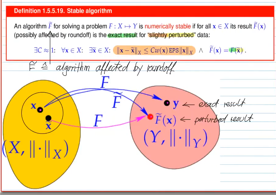
stable algorithm
Video 2.1
square LSE -> uniqueness of solution, if
(do not use matrix inversion function to solve LSE with numerical libraries)
Video 2.1.0.3
Video 2.2.2 Sensitivity/Conditioning of LSE
quantifies how small (relative) perturbation of data lead to changes of the output

condition of a matrix
if condition number of matrix is very large, it's columns/rows are almost linearly dependent (
Video 2.3 Gaussian Elimination (GE), LU-decomposition
- Gaussian eleminitaion ->
- LU-Decomposition ->
-> three-stage splitting of GE
X = A.lu().solve(B)
Video 2.6 Exploiting structure when solving linear systems
Video 2.7.1 sparse matrix: how to store
Video 2.7.2 sparse matrices in
Eigen
standard CRS/CSS format
#include<Eigen/Sparse>
Eigen::SparseMatrix<int, Eigen::RowMajor> Bsp(rows, cols);

#initalise
std::vector <Eigen::Triplet<double>> triplets;
Bsp.setFromTriplets(triplets.begin(), triplets.end());
alternative: allocate enough space at start (see 2.7.2.1) / squeeze out zeroes -> slightly more effizient than triplets, but the non-zero data size is not always known in advance
Video 2.7.3 direct solutions of sparse LSE (LGS)
mat.solve(vec);
// note: matrix is
Eigen::SparseLU<Eigen::SparseMatrix<double>> mat;
-> sparse solution is stable
(sparse elimination for combinatorial graph laplacian: asymptotic runtime
=> in practice: Cost(sparse solution of
Video 3.0.1 Overdetermined linear systems
Video 3.1.1 Least squares solution
idea: find vector
notation: lsq(A,b)
- least square solutions always exists
Video 3.1.2 solving least square problems
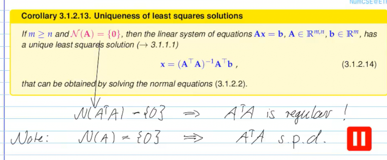
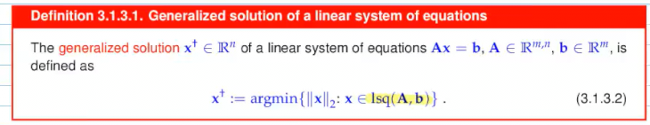
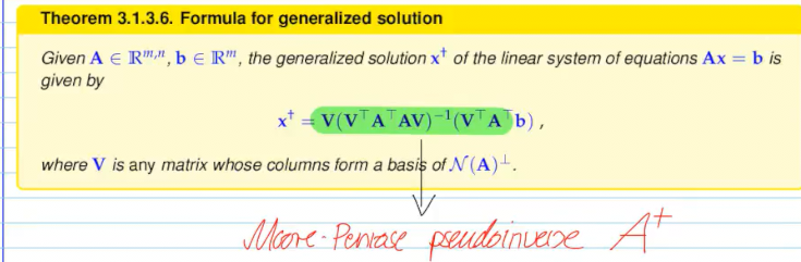
Video 3.1.3 Moore-Penrose-Pseudoinverse
LSQ solution not unique:
- FRC is violated
-> Additional selection criterium:
4.1 Filters and Convolutions
Video 4.1.1 Filters and Convolutions
discrete finite linear time-invariant casual channels/filters
- finite: it stops after some time
- time-invariant: the result does not change if it arrives now or 1min later
- linear: addition + multiplication with scalar
- casual: output only after onset of input
Video 4.1.2 LT-FIR linear Mappings + convolutions
- convolutions are commutative
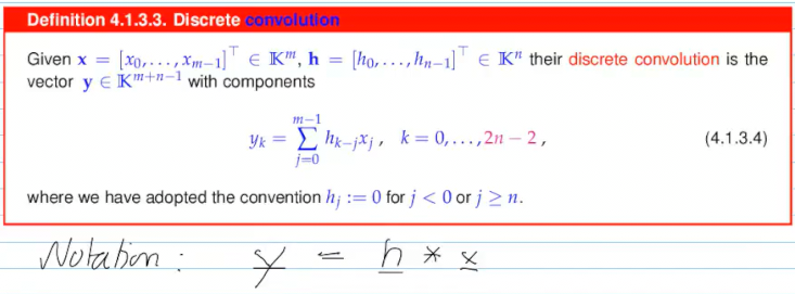
Video 4.1.3 Discrete Convolutions
Video 4.1.4 Periodic convolutions
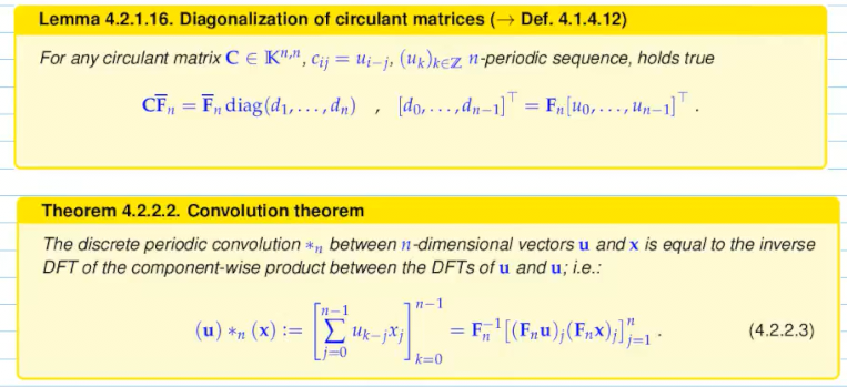
Video 4.2.1 Diagonalizing circulant matrizes
n-th root of unity
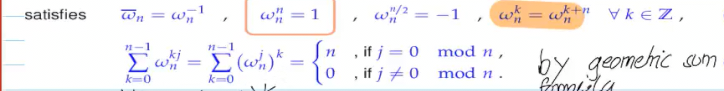
- the scaled fourier matrix
is unitary:
- the fourier matrix diagonalizes circulant matrices
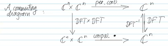
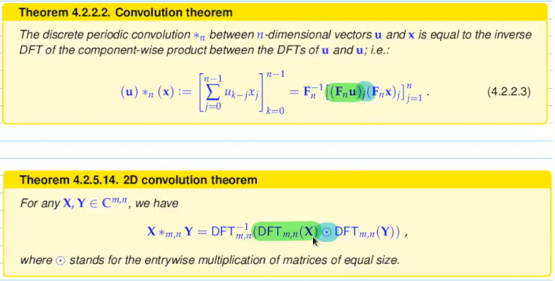
Video 4.2.2 Discrete Convolution via DFT
Eigen::FFT<double> fft;
fft.inv(
	(
		(fft.fwd(u)).cwiseProduct(fft.fwd(x))
	).eval()
)
explanation:
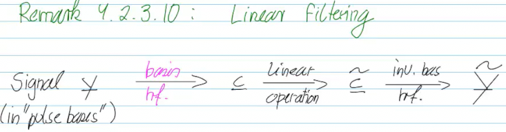
Video 4.2.3 Frequency filtering via DFT
Video 4.2.5 Two dimensional DFT
Video 4.2 FFT
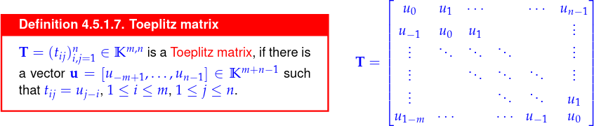
Video 4.5 Toeplitz Matrix Techniques
Toeplitz matrices:
- data sparse (not sparse)
Video 5.1 AI (Abstract Interpolation)
get unique solution
if
interpolant can be recovered by forming a matrix-vector product
#todo write down end of video
Video 5.2 Uni-Variate Polynomials
Polynomials form a Vectorspace with
convention for storing polynomials:
Video 5.2.2 Polynomial Interpolation Theory
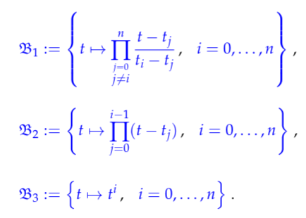
B1 - Lagrangian basis
B2 - Newton basis
B3 - monomial basis
Video 5.2.3 Polynomial Interpolation Algorithms
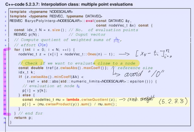
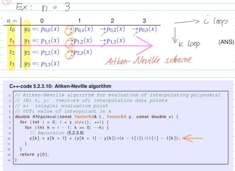
-> adding one more point (
Video 5.2.3.3 Extrapolation to Zero
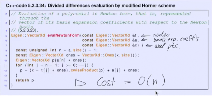
Video 5.2.3.4 Newton Basis
Homer-like scheme
Video 5.2.4 Polynomial Interpolation: sensitivity
sensitivity: amplification of perturbation of data (of a problem)
-> tiny errors will have huge impact on the interpolation result
-> not suitable for data interpolation
6. Approximations of functions in 1D
Video 6.1 Introduction
in 5: create function to combine data points
in 6: find easier function, because 5 too costly
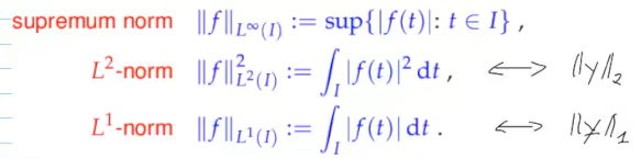
-> find simple (easy to evaluate) function with small approximation error (norm)
Video 6.2.1 Polynomial approximation: theory
bernstein theorem: if
- but not how close, how fast -> dissapointing
jackson theorem: Max-norm of best-approximation error
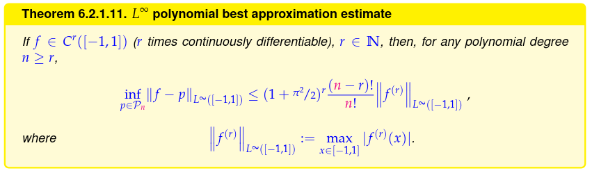
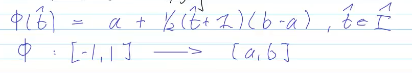
how to move from interval
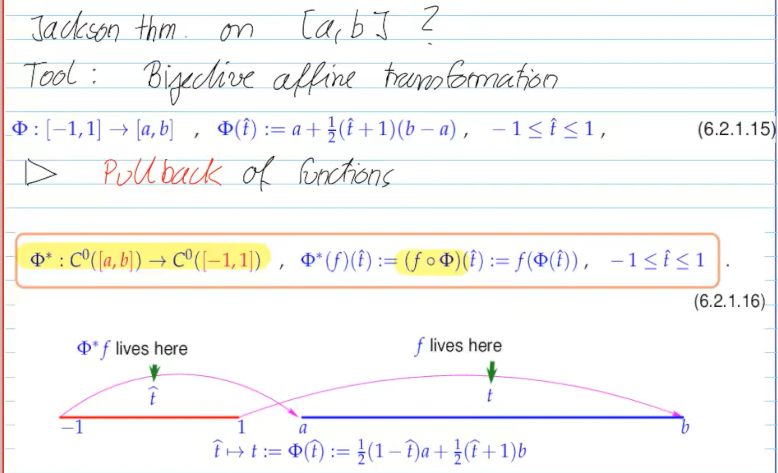
- max norm stays same
- perserves degree of polynomials
- derivative: change uniformly
Video 6.2.2 Convergence of interpolation errors
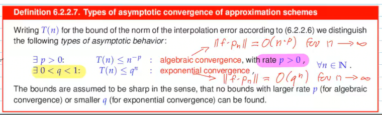
what can you tell from algebraic divergence?
-> how to increase polynomial degree to achieve certain reduction of error
Video 6.2.2.2 Interpolands of finite smoothness
Runge's Counterexample:
Video 6.2.2.3
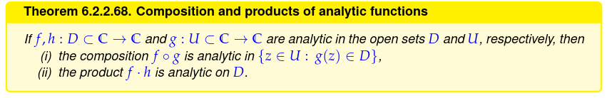
real analytic function
-> if has convergent taylor series for every point in interval
Video 5.2.3.1 Chebychev Interpolation
The
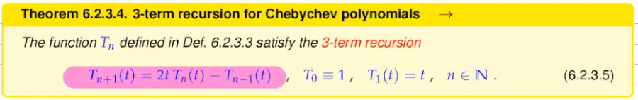
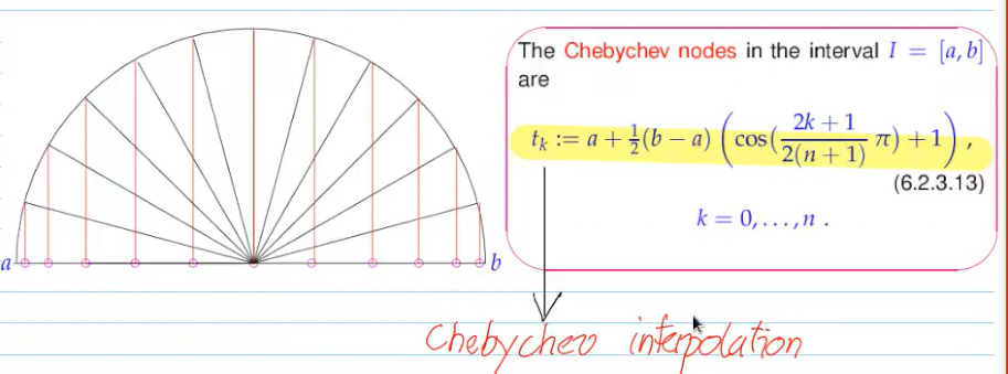
Video 5.2.3.2 Chebyshev INterpolation Error Estimates
equidistnt nodes affected by oscillations close to endpoints
Lebeseque links best approximation error and interpolation errors
Lebesque constant for Chebychev nodes:
-> increase verys slowly
(compare with equid. nodes:
trick: plug in lebesque constant in between interpolation error and best approximation error

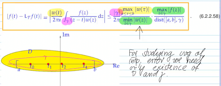
Suitebla integration path: elippsis around
-> cos, to cancel out with chebyshev polynomials
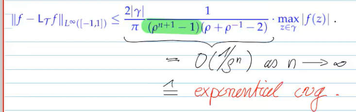
for chebyshev polynomials for analytic functions
slower for smaller domain of analyticity
Video 6.5 Approximation by Trigonometric Polynomials
space of 1-periodic functions of trigonometric functions of degree 2n
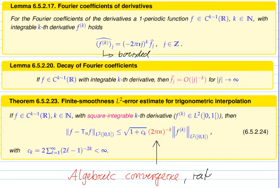
Video 6.5.2 Trigenometric Interpolation Error Estimates (fourier series)
#todo didn't quite understand the video
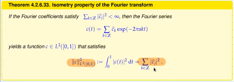
->
Video 6.6.1 Piecewise Polynomial Lagrange Interpolation
approximation by piecewise polynomials
piece-wise polynomials; benefit:
- locality
- cheap algorithm
- shape preservation
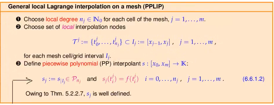
lagrange interpolation for function that is
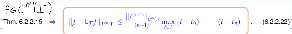
for mesh width
7. Numerical Quadrature
Video 7.1 Introduction
Numerical Quadrature (Integration)
7.2 Quadrature Rules
Video 7.2 Quadrature Formulas Rules
double f(double)
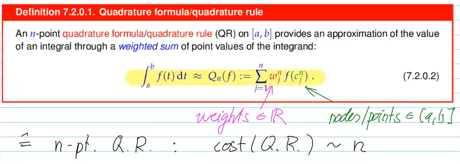
transformation:
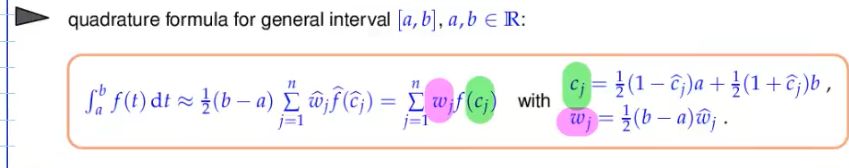
interpolation schemes (5) -> approximation schemes (6) (simple functions) -> quadrature schemes (7)
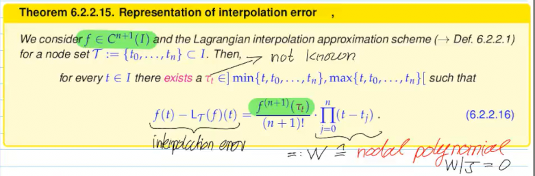
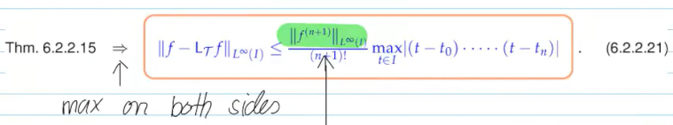
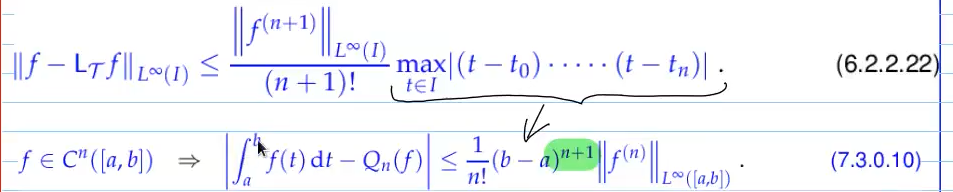
quadrature erros can often be computer easily, especially for quadrature rules arising from interpolation schemes
(bounded by max norm of interpolation error)
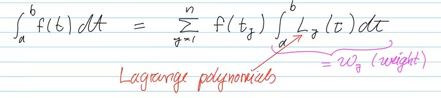
7.3 Polynomial Quadrature formulas
Video 7.3 Polynomial Quadrature Formulas
Use Lagrangian polynomial interpolation
- midpoint rule
- trapezoidal rule
Dangerous for
solution:
- chebyshev nodes -> no cancellation, since weights
error estimates for polynomial quadrature:
7.4 Gauss Quadrature
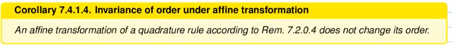
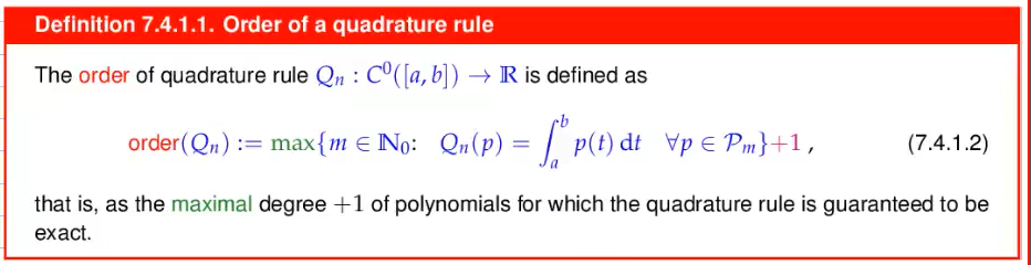
Video 7.4.1 Gauss Quadrature / Order of a Quadrature Rule
order of polynomial n-pt. quadrature rule = n, since n-1 polynomail -> n+1 of that order of quadrature rule
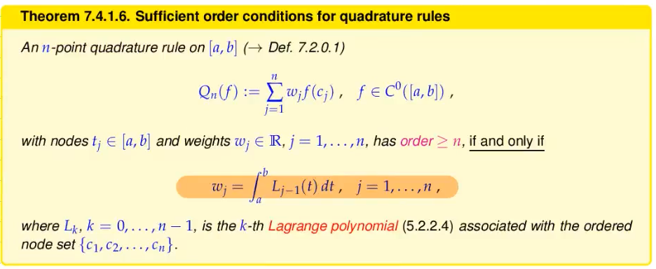
7.4.1.7: how to compute weights to achieve order n by solving a suitable linear system:
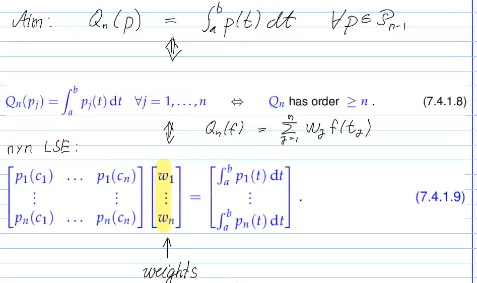
-> solve weights to get quadrature rule of at least order
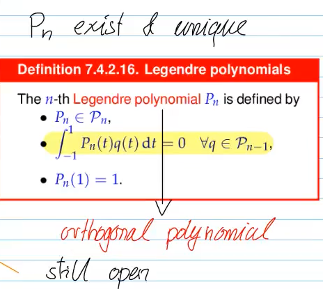
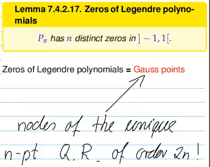
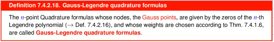
Video 7.4.2: Maximal-Order Quadrature Rules
how to find maximum order quadrature rule?

how to find n-point quadrature rule of order 2n?
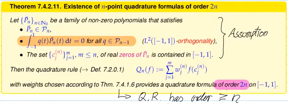
Note that Hiptmair mostly proves lemmas indirectly.
Video 7.4.3 Quadrature Error Estimates
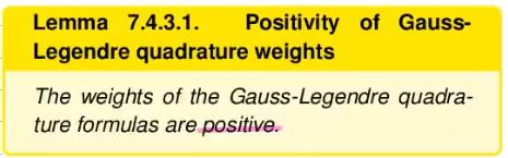
very important property for quadrature error:
from chapter 6);
- limithed smoothness of f: (
, but ):
algebraic convergence with rate r () - analytic
-integrand (analytic extension):
exponential convergence ()
restoring smoothness (removing singularity by transformation):
- integration by substitution (e.g.
-> gets analytic) (more art than science, but can often be used)
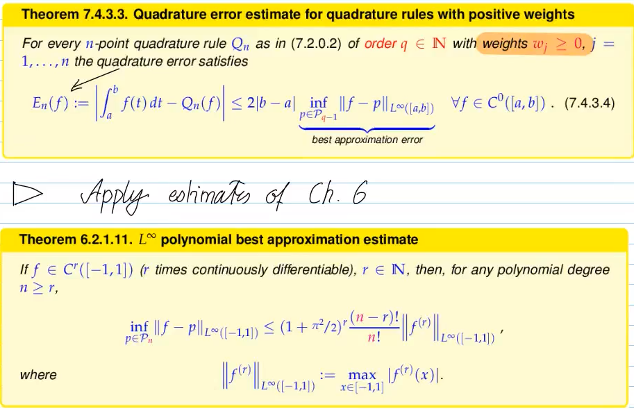
The message of asymptotic estimates:
- tell us how much additional work ~ n is needed to reduce Error by factor
- algebraic convergence:
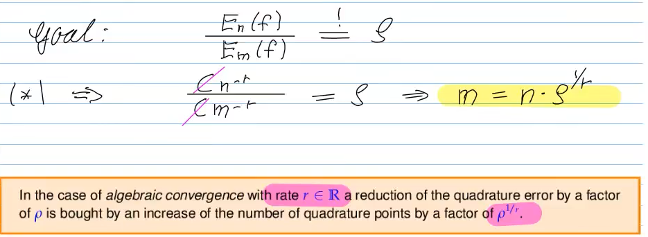
- exponential convergence:
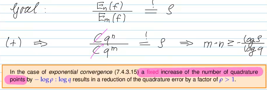
-> adavantage of exponential convergence: needs fixed amount of points to reduce error by factor
Eigen::ArrayXd::LinSpaced(n,a,b)
builds a sequence of
Video 7.5 Composite Quadrature
split interval into mesh, integrate very mesh individually
-> cost = number of mesh cells (* integral)
good approximation for local error:
"h-covergence": convergence by making mesh finer
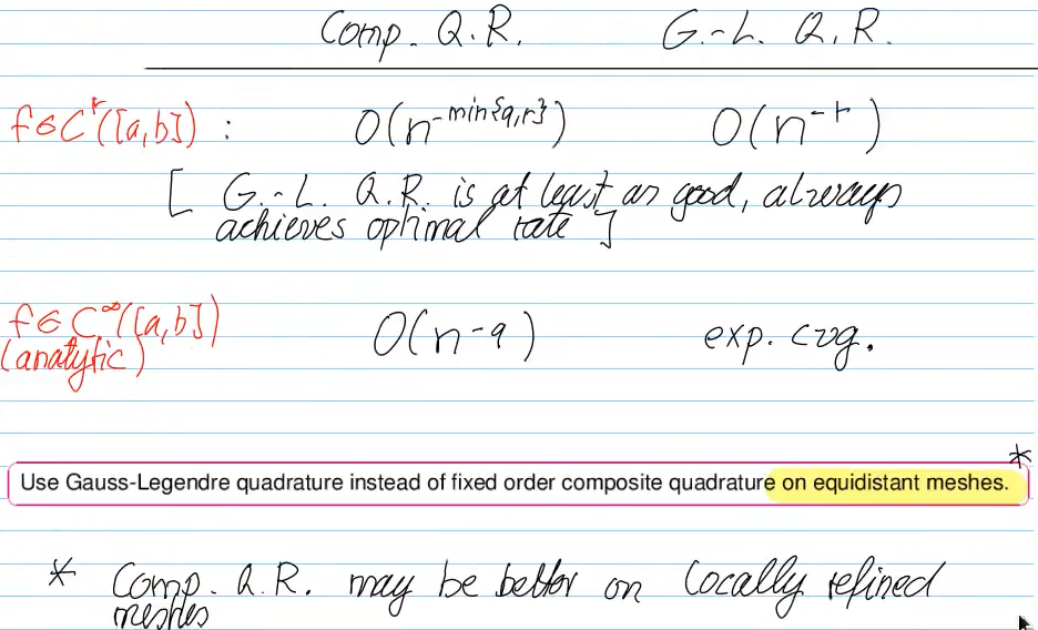
-> for equidistant meshes, use Gauss-Legendre Q.R. instead of composite quadrature
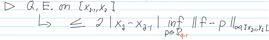
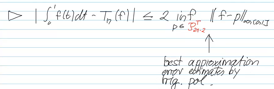
-> for trigonometric polynomials (periodic functions):
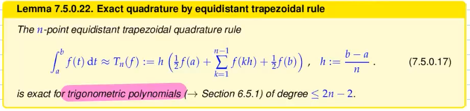
with
best approximation error estimeted by triag.pol.:
Video 7.6 Adaptive Quadrature (13 min)
goal: choosing mesh such that local errors are equidistribution
-> choose mesh a priori (based on prior knowledge about f) (often not known)
-> choose mesh a posteriori (automatic based on informatio gained during the computation)
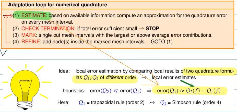
with initial mesh
- compute estimate for each mes cell: (simpson - trepezoidal Q.R.)
- sum up to get estimate for total error
- if error too large, find intervals contribute above average to the total error
- add their midpoints to the new refined mesh. start anew.
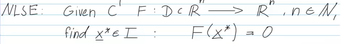
8. Iterative Methods for Non-linear Systems of Equations
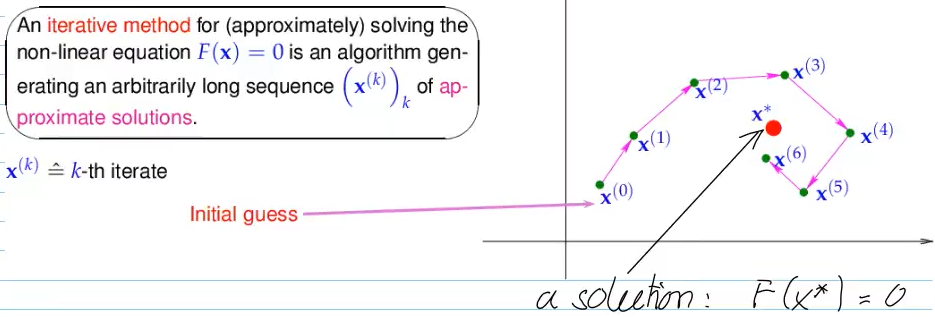
Video 8.1 Iterative Methods for Non-Linear Systems of Equations: Introduction (5 min)
form:
- n number of unknowns/equations
- no general theory
- F often only implicit
8.2 Iterative Methods
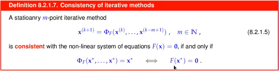
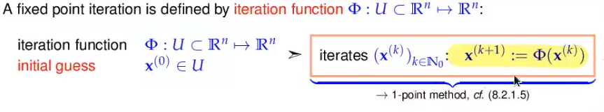
Video 8.2.1 Fundamental Concepts (6 min)
solve by "getting closer and closer" iteratively
-> will this solution converge?
m-point method:
-> insert last
- start with initial
guesses:
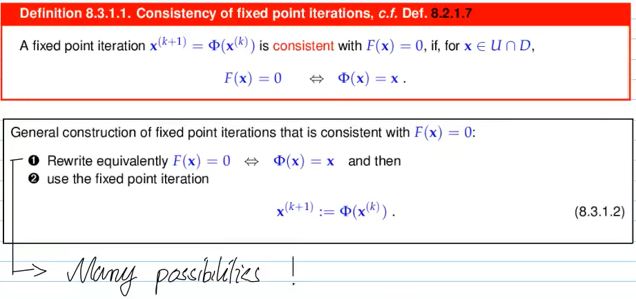
consistent: vector at which iteration becomes stationary -> vector must be solution
-> consequence: assume
- limit of sequence exists (
cvgt.) - iteration function consistent (
consistent) - iteration function continuous on all arguments (
continous)
=>
local convergence:
- cvg. will heavily depend on initial guess
- how fast will the convergence of the sequence
solution be? 8.2.2 - what is the initial region of local convergence?
partially answered by 8.3
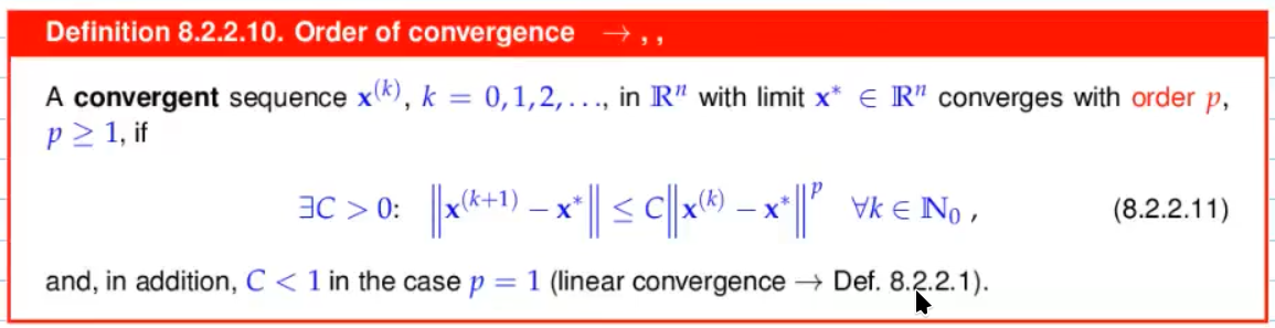
Video 8.2.2 Speed of Convergence (15 min)
How fast will the norm converge?
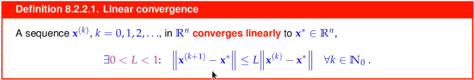
smallest L: rate of cvg.
Detect linear convergence:
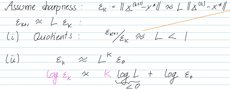
- p=1 -> linear convergence
- C usually unknown
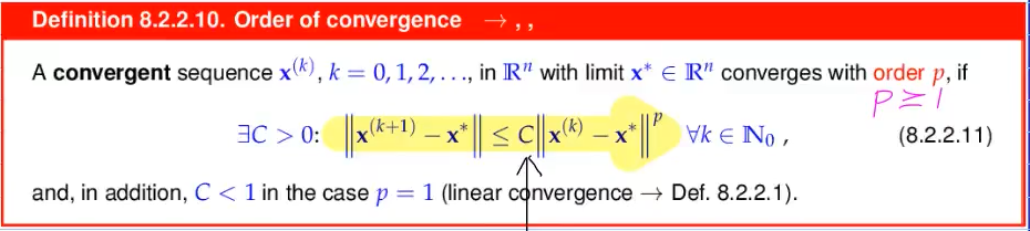
Detect p
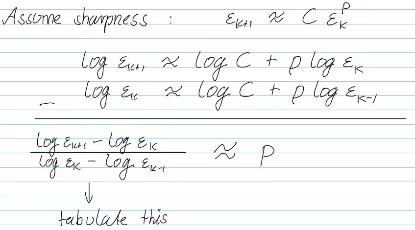
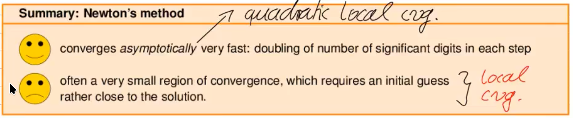
quadratic convergence (p=2): doubling of correct digits in each step
Video 8.2.3 Termination Criteria/Stopping Rules (14 min)
Ideal stopping rule:
stop iteration if prescribed absolute or relative tolerance reacher
-> not working, since exact value not known
practical stopping rules
- A priori termination -> STOP after a fixed no. of steps
- Residual-based termination -> STOP, when
prescribed tolerance - tells us little about
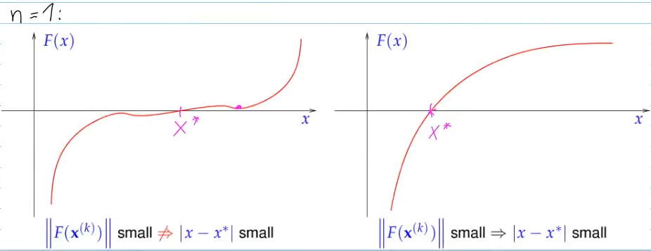
- tells us little about
- Correction-based termination -> stop convergent iteration, when correction stops changing much
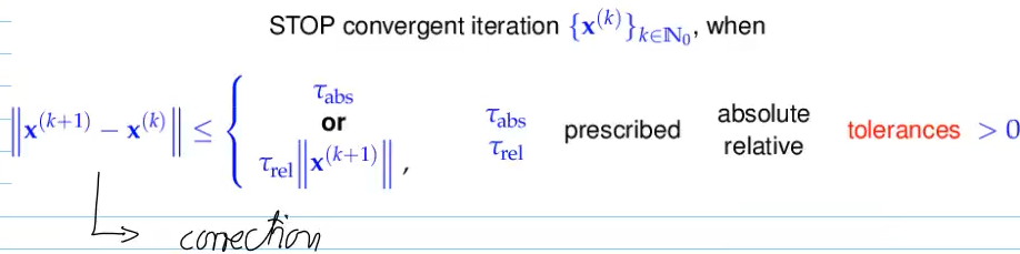
error estimate:
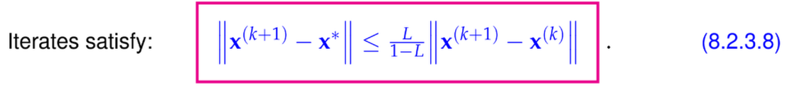
-> Reliable error estimate, even if we only know upper bound
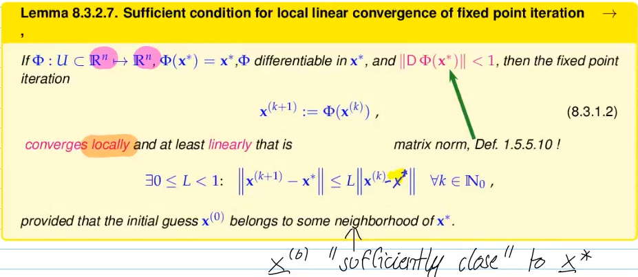
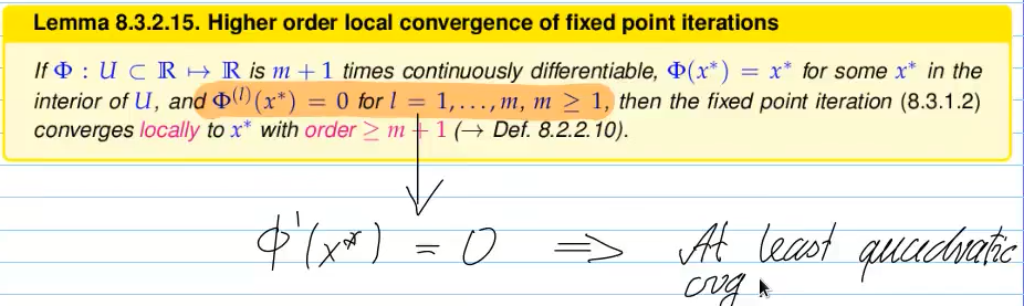
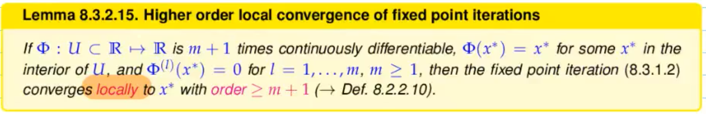
8.3 Fixed-Point Iterations
Video 8.3 Fixed-Point Iterations (12 min)
we do not always know
Video 8.4.1 Finding Zeros of Scalar Functions: Bisection (6 min)
find
If on interval
Idea: geometrically decrease interval
-> linear convergence, factor
+ guaranteed cenverence -> robust
+ F - only evluations needed -> procedural ok
+ derivative-free
+ works
- not extremely fast
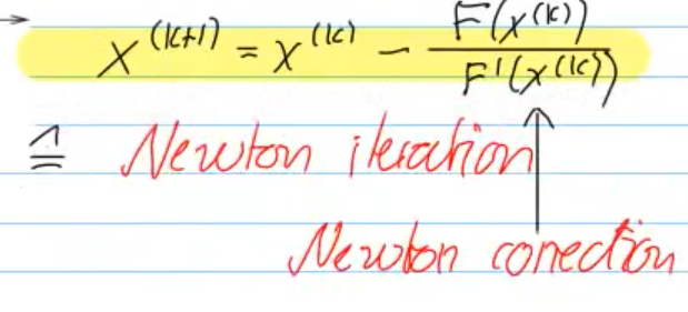
Video 8.4.2.1 Newton Method in the Scalar Case (20 min)
Idea: replace function locally around
Newton: use tangent on
Ex. 8.4.2.4: functions with same
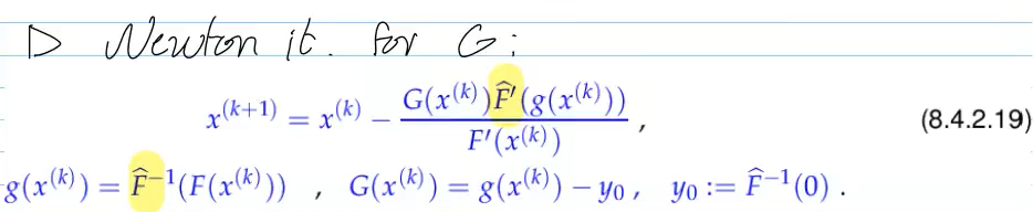
Find
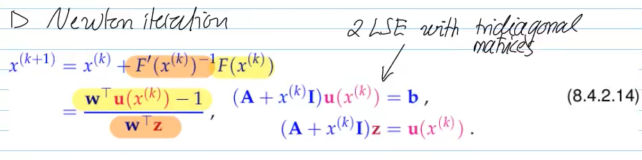
If (F) is hard to solve but close to an easily invertible
Then
Newton on (G) converges faster and from farther away because the preconditioning makes the problem closer to the identity map.
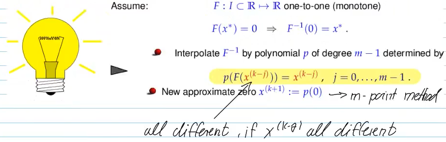
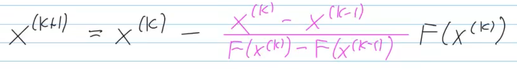
Video 8.4.2.3 Multi-Point Methods (12 min)
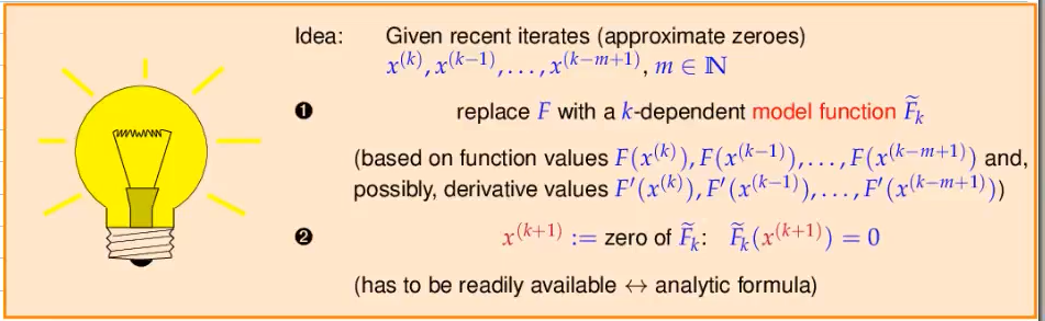
secant method:
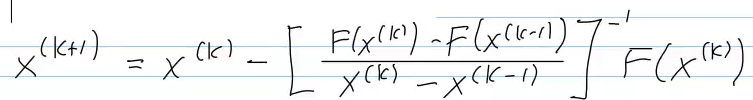
- replaces derivative in Newton's method by quotient
- 2-point method, requires 2 initial guesses
- derivative-free
- one F-evaluation per step
- if function flat, breaks down
- fractional convergence with p
1.62
-> secant method more efficient (see 8.4.3) than Newton method!
8.4 Finding Zeros of Scalar Functions
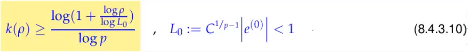
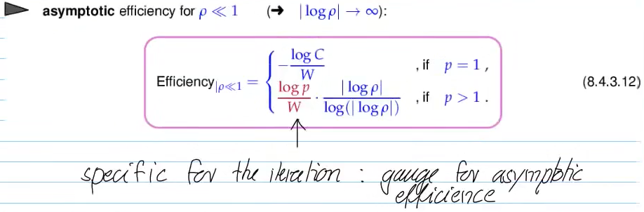
Video 8.4.3 Asymptotic Efficiency of Iterative Methods for Zero Finding (9 min)
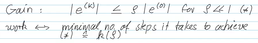
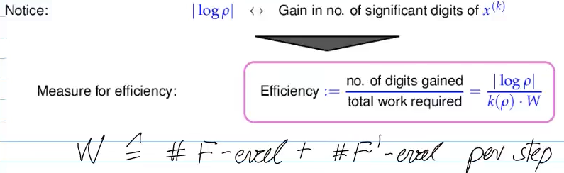
lower bound for number of required steps:
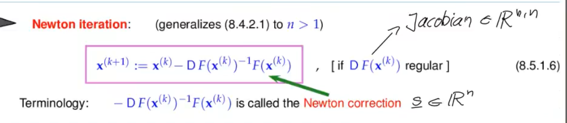
8.5 Newtons Method in
Video 8.5.1 The Newton Iteration in Rn (I) (10 min)
The standard method for solving (generic) non-linear systems of equations.
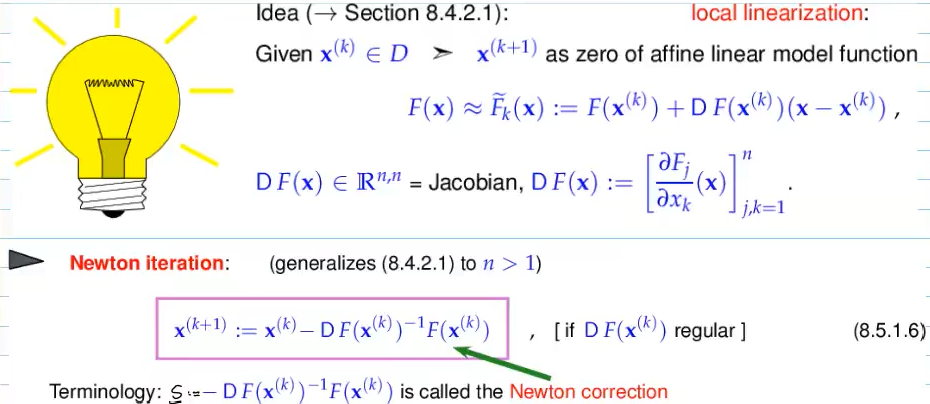
Newton method if affine invariant (invariant to multiplicaiton with matrix from left)
-> should also be desireable for stopping rules
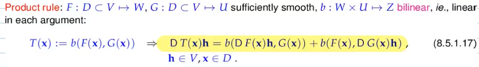
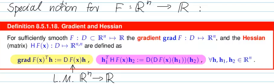
Video 8.5.1.15 Multi-dimensional Differentiation (20 min)
Matrix * Vector is general way to write linear mapping
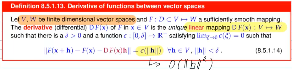

bilinear

Video 8.5.1 The Newton Iteration in Rn (II) (15 min)

Simplified Newton method:
- Drawback: usually sacrifices the asymptotic quadratic convergence of the Newton method: merely linear convergence can be expected.
#todo look video again to understand better
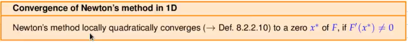
Video 8.5.2 Convergence of Newton’s Method (9 min)
Convergence of Newton's method:
Video 8.5.3 Termination of Newton Iteration (7 min)
terminate, when
=>
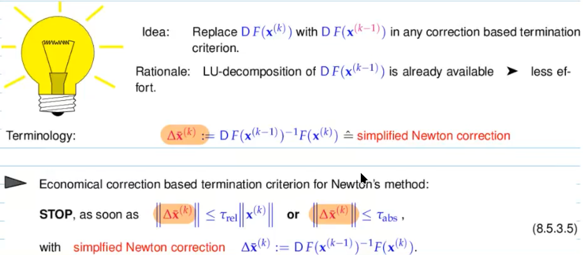
-> affine invariant: does not change when
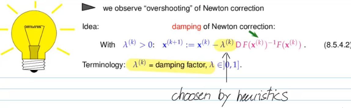
Video 8.5.4 Damped Newton Method (11 min)
=> goal: enlarge domain of cvg.
- Newton correct in the wrong direction -> no remed
- "Overshooting" Newton correction -> apply damping
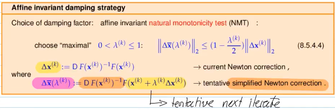
if quadratic cvg. =>
if NMT (natural monotonicity test) fails
& retry
if passed- next step, (8.5.4.2),
in next step
-> works, because of affine invariant property of Newton method
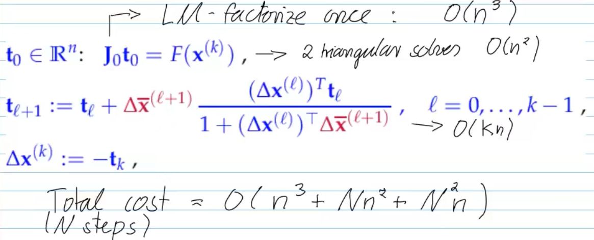
8.6 Quasi-Newton Method
Video 8.6 Quasi-Newton Method (15 min)
Drawback of Netwon method: DF required
- Goal: Derivative-free iteration of NLSE
- for
: Secant method, 8.4.2.3
- replaces
(Jacobian) with difference quotient approximation
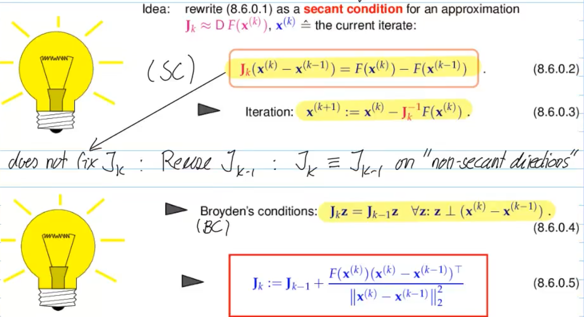

- No asymptotic quadratic cvg. for Broyden's quasi-Newton method (but still faster than e.g. simplfied Newton)
- rank-1-modification
for
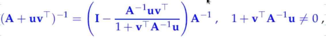
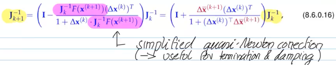
- solve
LSE - vector arithmetic from then on (very cheap)
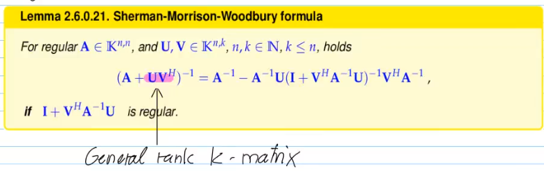
can have stability problems! (because of SMW-formula)
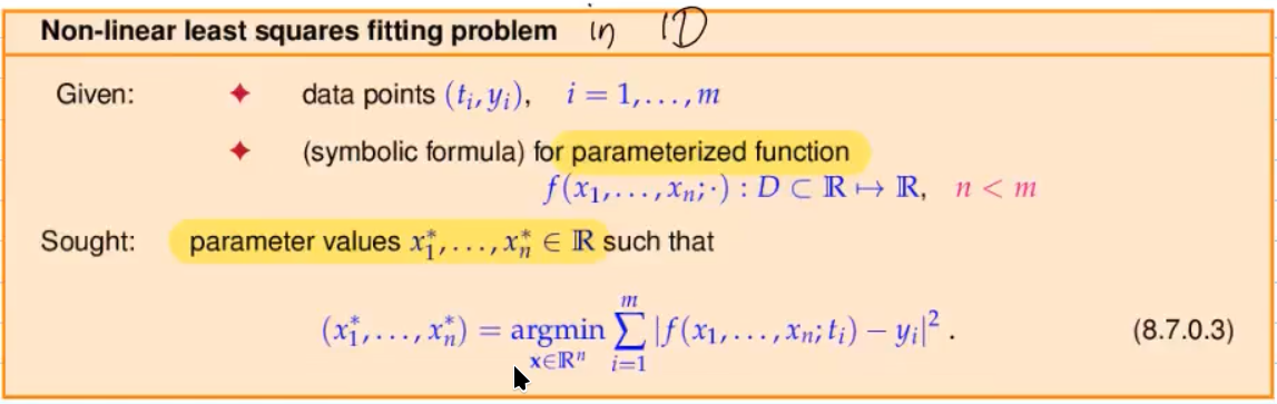
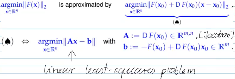
8.7 Non-linear Least Squares
Video 8.7 Non-linear Least Squares (7 min)
minimize Euclidean norm of residual (same as linear case)
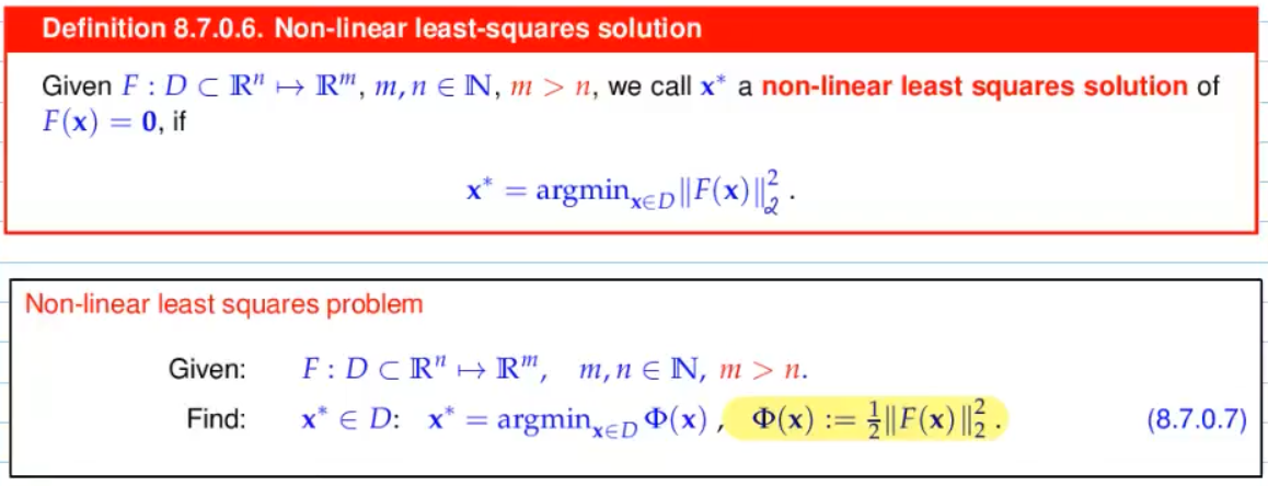
- forefactor
only convention - More general version of the linear least squares problem
linear case:

linear combination of basis function
non-linear case:
Video 8.7.1 Non-linear Least Squares: (Damped) Newton Method (13 min)
with
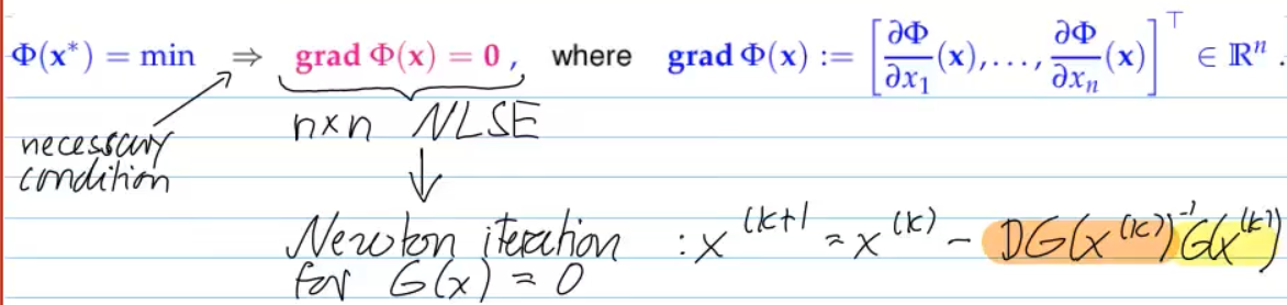
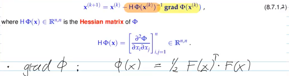
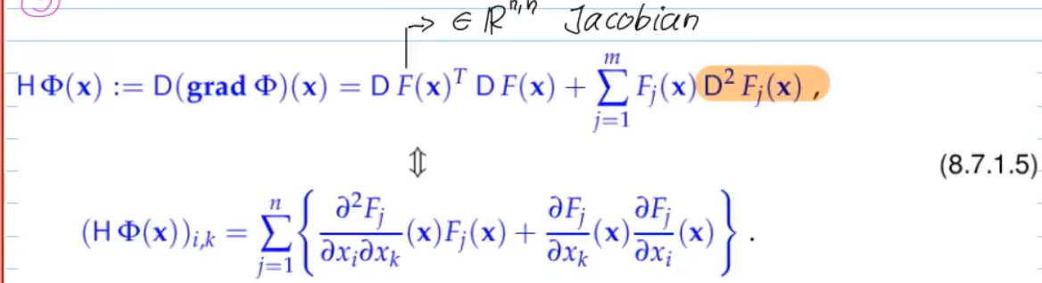
then the LSE for Newton crrection
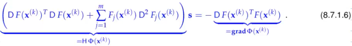
-> normal equation in case
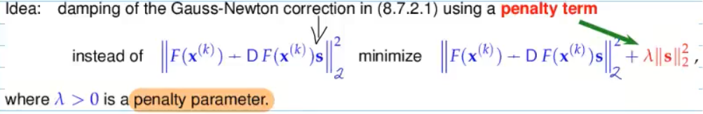
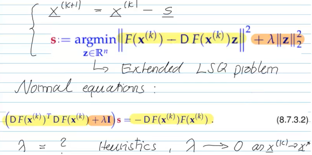
Video 8.7.2 (Trust-region) Gauss-Newton Method (13 min)


Advantages over Newton-method:
+ 2nd-derivativ free
+ Larger domain of cvg.
- no local quadratic cvg.
-> no global cvg., but we can also use damping (called trust region Method
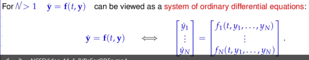
11. Numerical Integration - Single Step Methods
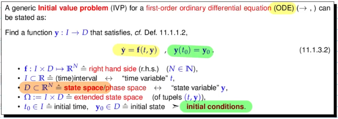
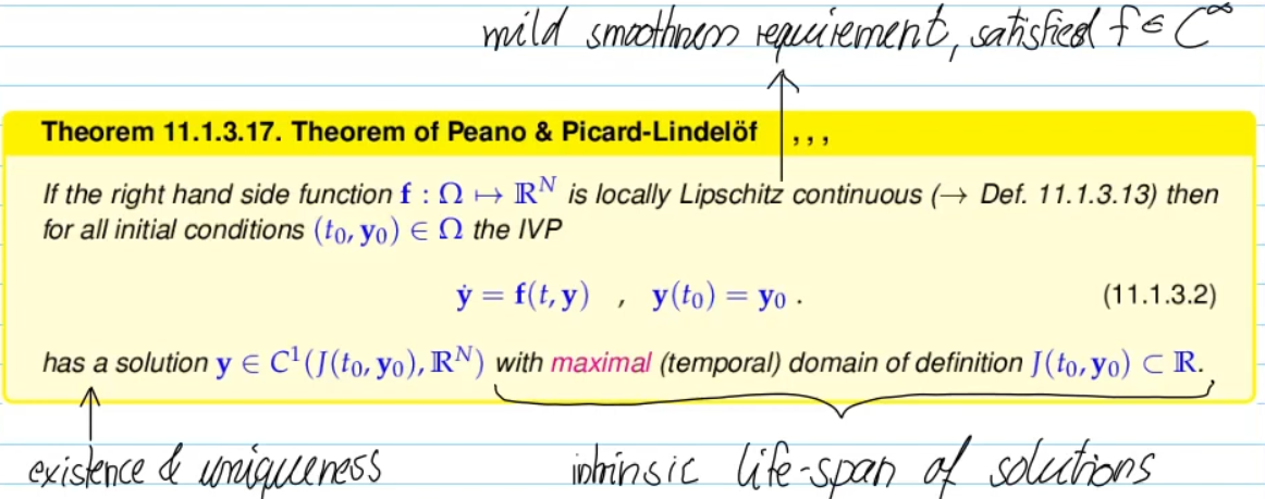
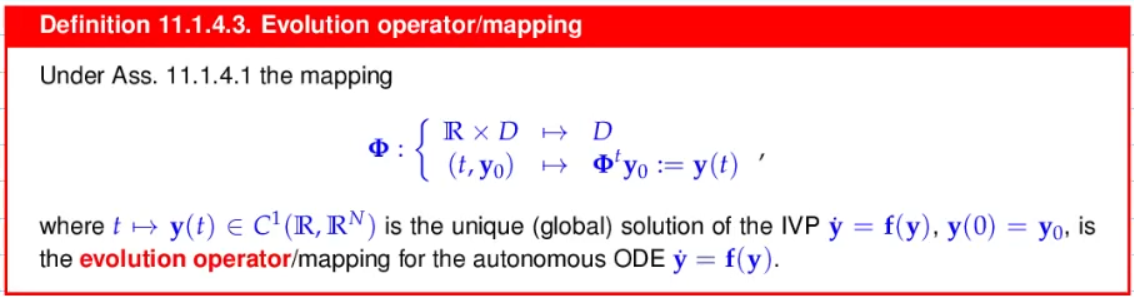
Video 11.1 Initial-Value Problems (IVPs) for Ordinary Differential Equations (35 min)

- for autonomous ODE, choosing initial time
is natural - time invariant -> wa can always fix initial time
without loosing generality
time-dependent ODEs can be converted to autonomous ODEs
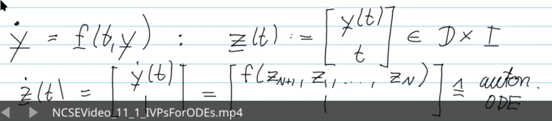
conversion: from higher-order ODEs for first-order ODEs
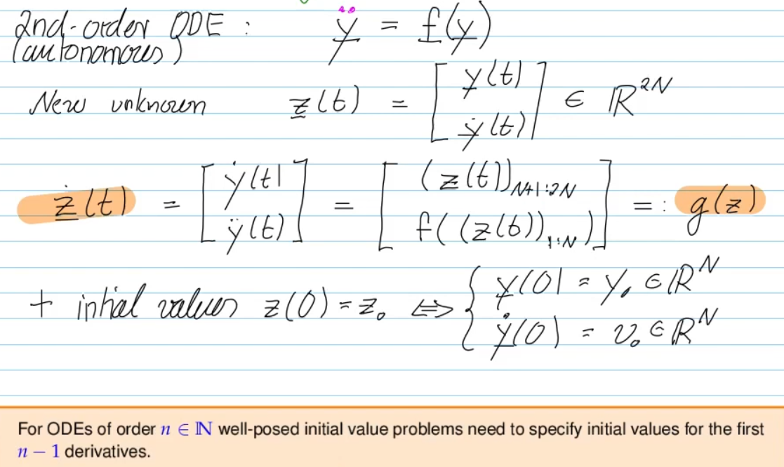
- for initial-value problem, we have to specify initial values for both
for the first-order ODE

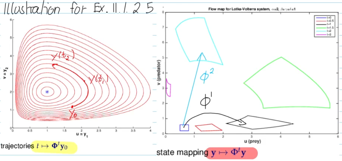
left:
- trajectory of single initial point moving through space
- fix starting point, vary time
right:
- a set of points move through space, with evolution operators
- time fixed, look how all spatial points move
=> as time progresses, the evolution operator takes a "part of the space" and "flows" it forward
Recovering the ODE from the Flow: the vector field
- for Autonomous ODE, we have the group property:
11.2 Introduction: Polygonal Approximation Methods
11.2 Introduction: Polygonal Approximation Methods (17 min) (17.3 min)
explicit Euler method
- replace
with diff. quot anchored on M - explicit: no calculation, only evaluation at points:
implicit Euler method
- backwards diff. quotient instead of forwards diff. quotient
- feasible? -> continuity argument: for
solution should still exist
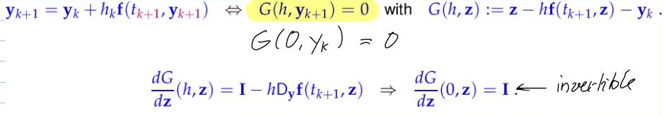
For sufficiently small
implicit midpoint method
again: replace
- symmetric diff. quot., halfway between
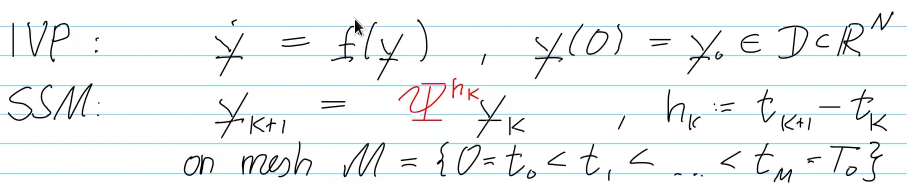
11.3 General Single-Step Methods
Video 11.3. General Single-Step Methods (14 min)
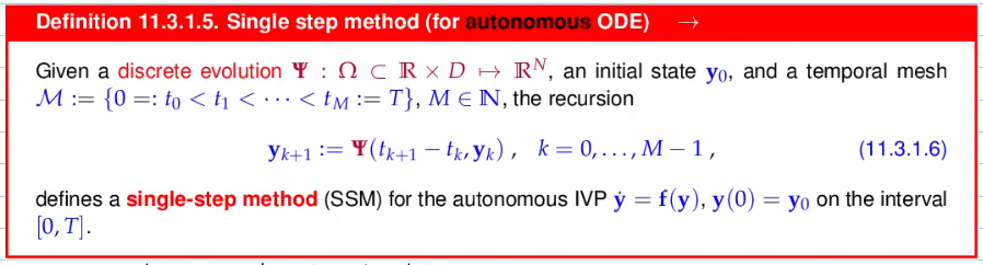
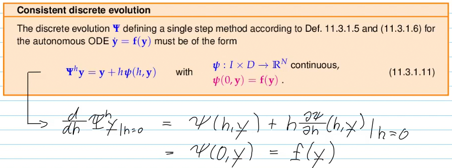
=>
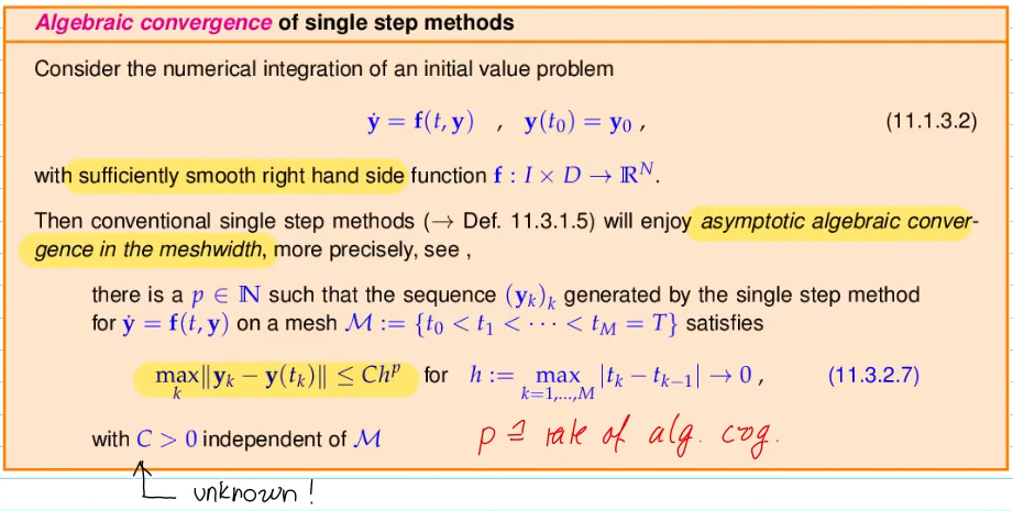
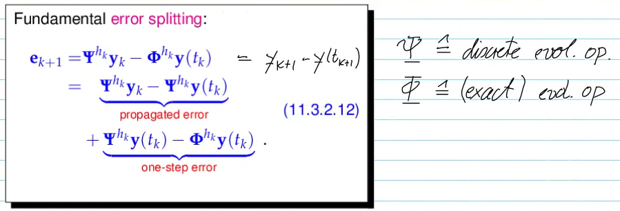
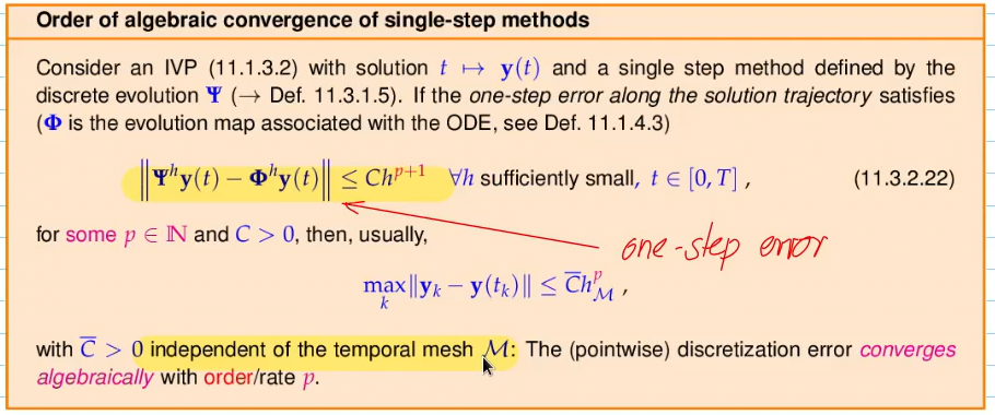
Video 11.3.2 (Asymptotic) Convergence of Single-Step Methods (20 min) (~30min)
... for the sake of simplicity, but without loss of generality ...
<repetition> (from [7.4.3.12])
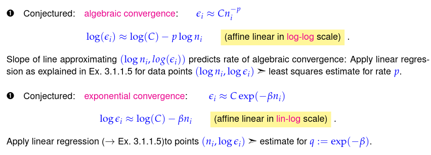
algebraic convergence
- line in log-log plot
exponential convergence
- line in lin-log plot (?)
</repetition>
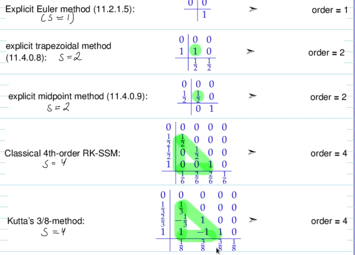
explicit/implicit Euler method:
- algebraic convergence with order 1
for
implicit midpoint method
- alg. cvg. with rate 2
for max point-wise error, we observe decay like

- explicit/implicit newton method: order 1
- implicit midpoint method: order 2
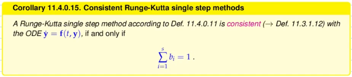
- Remains valid for all consistent SSMs:
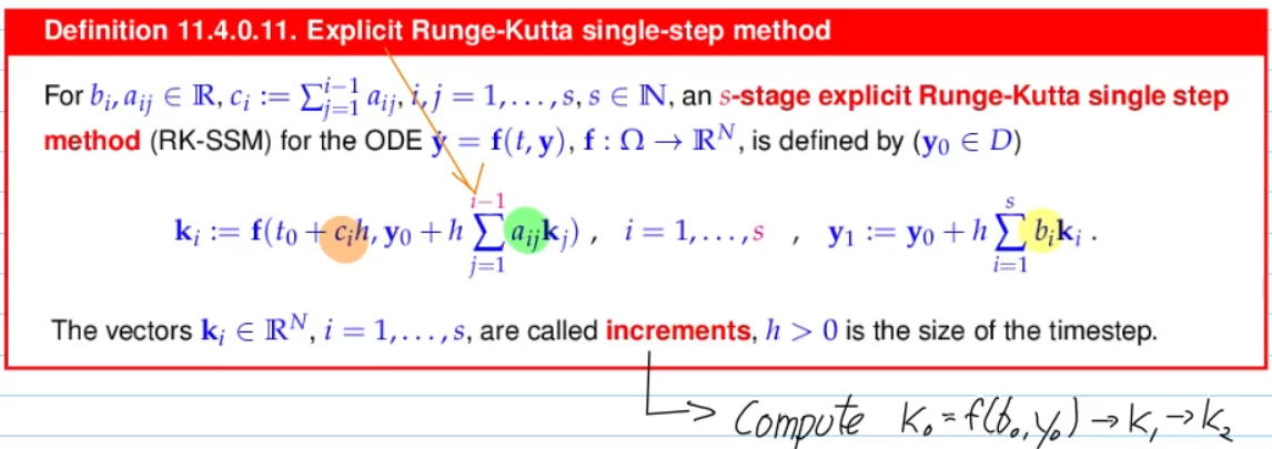
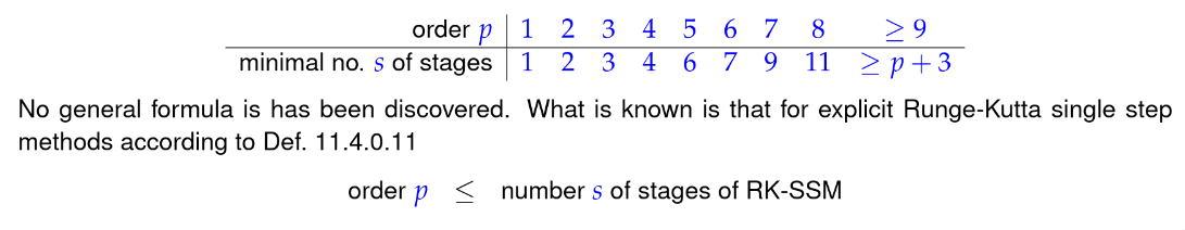
11.4 Explicit Runge-Kutta Single-Step Methods
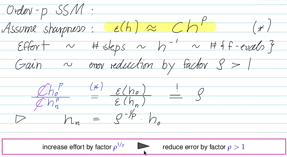
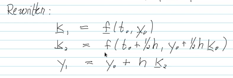
Video 11.4 Explicit Runge-Kutta Single-Step Methods (27 min)
Questions we can answer:
- How much additional effort do we have to invest for a desired gain (in accuracy)?
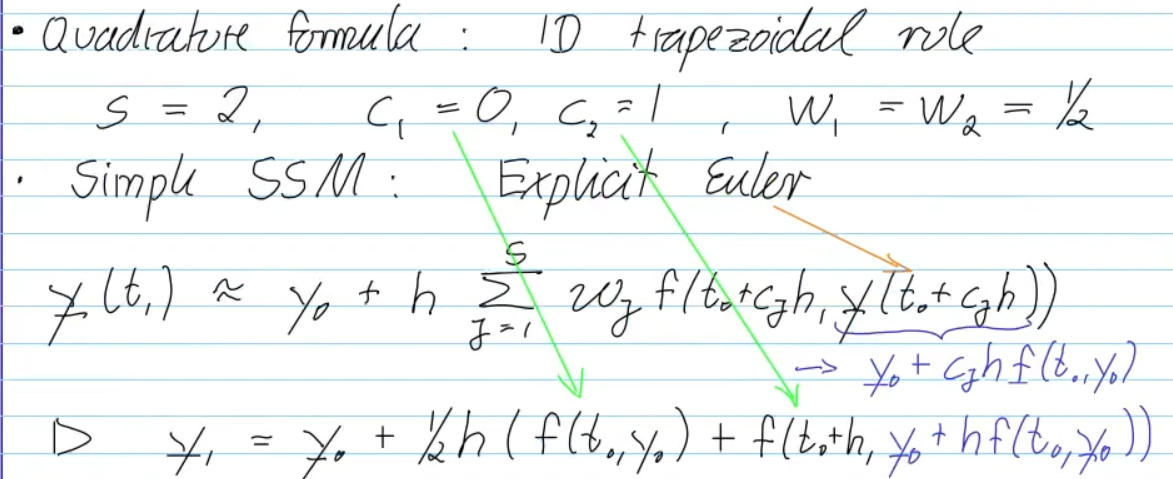
explicit trapezoidal method
- no solution of equs. required
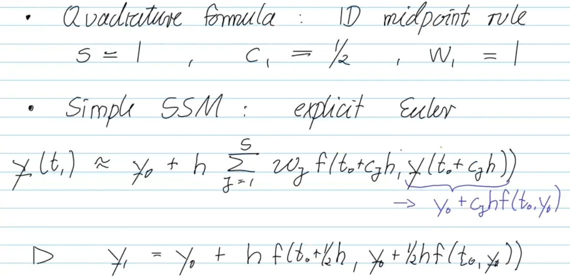
explicit midpoint method

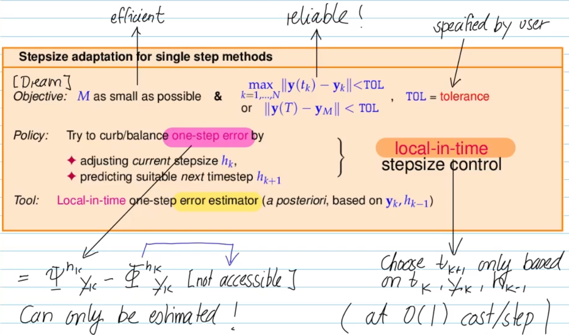
Video 11.5 Adaptive Stepsize Control (32 min)
<repetition>
<repetition>
abs. tolerance is safeguard if we encounter a zero-state
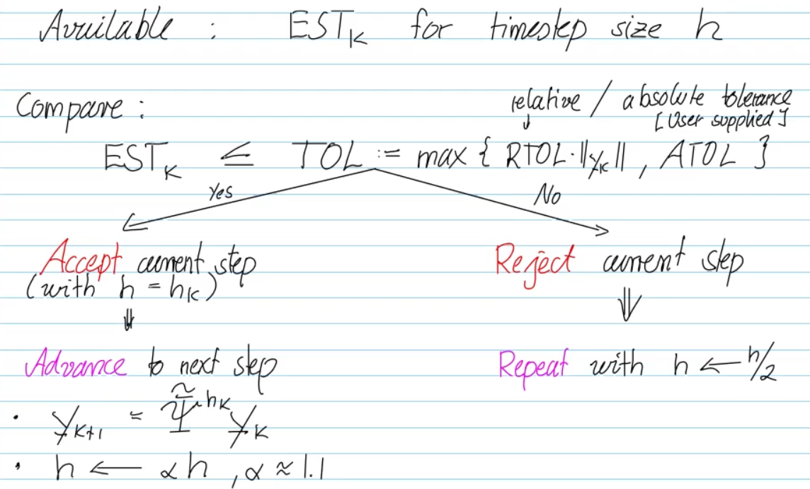
adaptive timestepping
- stable (always)
- can "fail", have even larger errors than uniform mesh, if the initial "large" steps accumulate many errors before we get to the fine mesh step part
refined local stepsize control:
- find "optimal" timestep -> largest possible timestep b.c. of efficiency
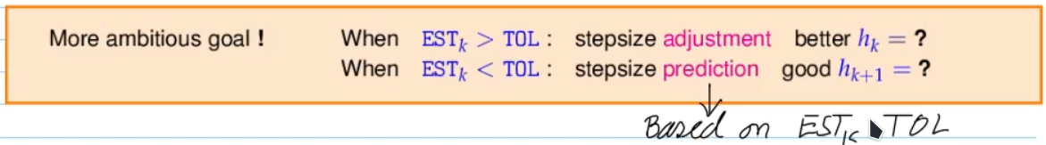

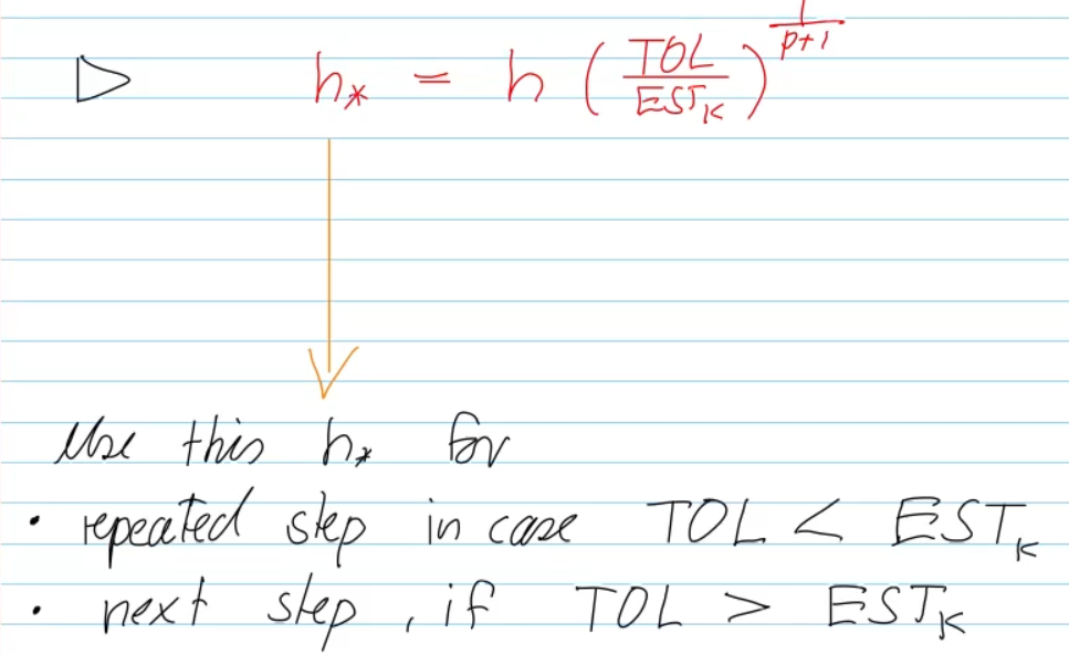
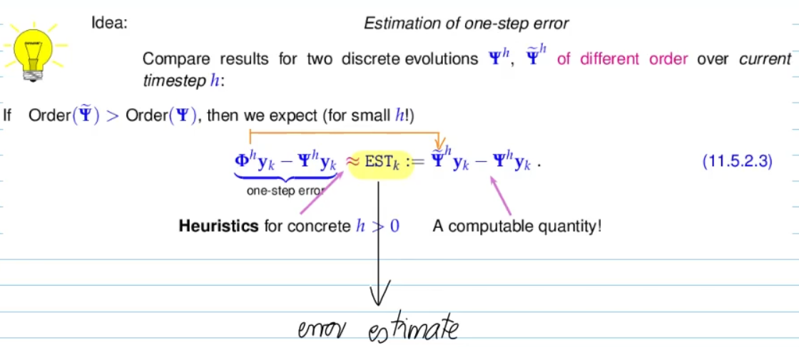
derivation:
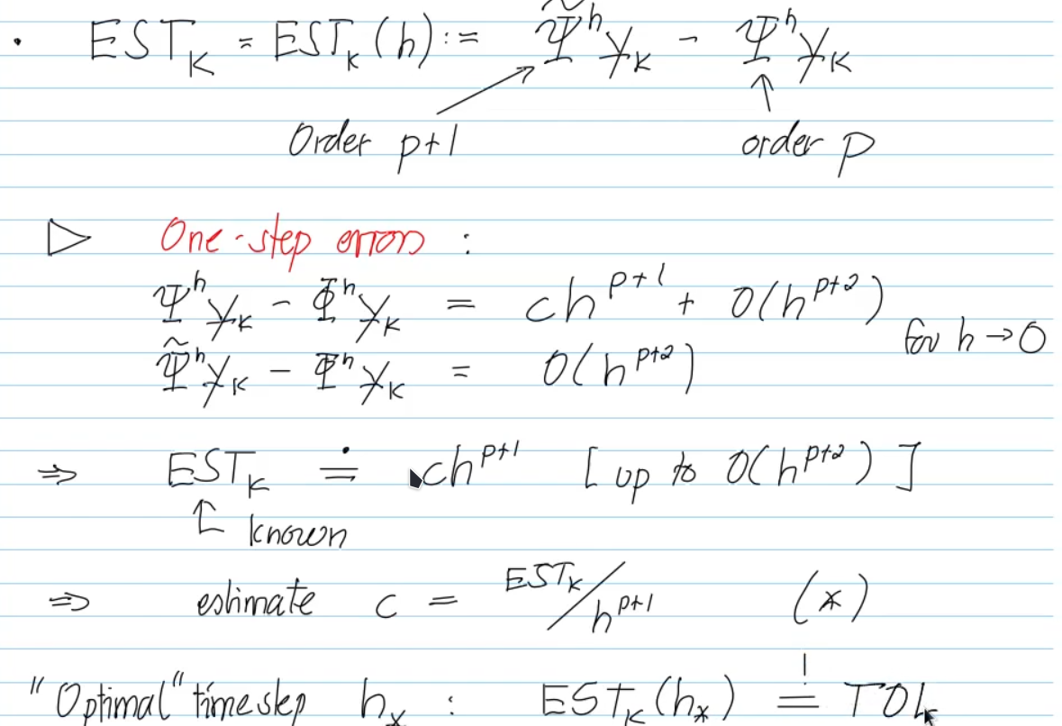
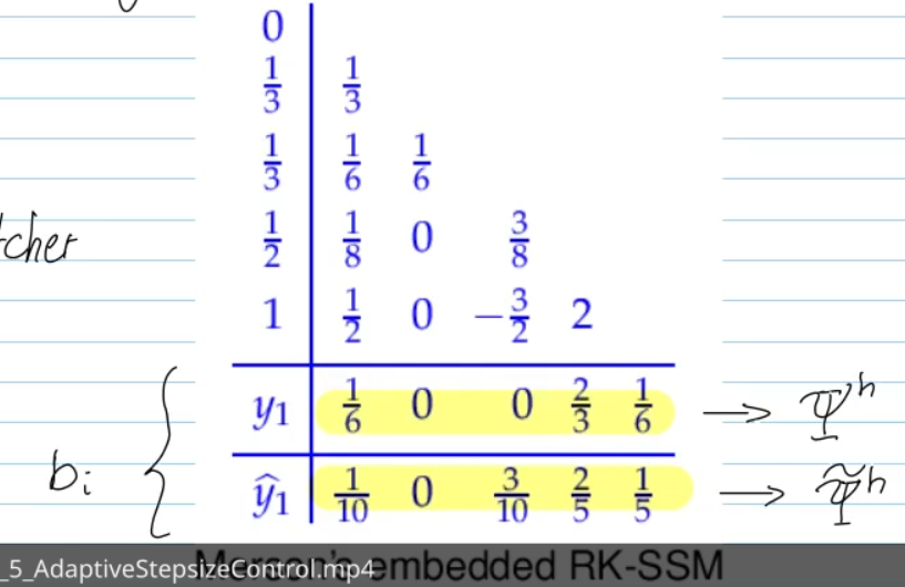
embedded runge-kutta methods:
- Idea: use same increments
, but with different weights -> is (high-order) p+1 method

-> inparticular for IVPs with sensitive dependence on initial conditions (exp 11.5.2.10) - b.c. one-step error is only loosly connected to discretization error
Video 12.1 12.1 Model Problem Analysis (40 min)