ETH_NumericalMethodsForCSE

Info

Doebel: https://publish.obsidian.md/ddoebel/Welcome
Dragos: https://polybox.ethz.ch/index.php/s/jgGpEyX6Ctf2KCD
- uploads faster than Popa
Popa: https://polybox.ethz.ch/index.php/s/roTjs6ppjc5fXW3
- (outdated: https://n.ethz.ch/~iopopa/)

all exercise slides:

NumCSE_exercise_sessions_merged.pdf

Übungen

#timestamp 2025-09-19

![[NumCSE_week1_practice.cpp]]

#timestamp 2025-10-03

why squared loss?

differentiable
always positive
icreasesquadratically with distance

(-> but sth. oder would also be possible)

least square solution:

\begin{aligned} (α, β) & = a r g m i n \sum_{i = 1}^{m} | y_{i} - α x_{i} - β |^{2} \\ = a r g m i n L (α, β) \\ \frac{\partial L}{\partial α} & = \sum_{i = 1}^{m} 2 (y_{i} - α x_{i} - β) (- x_{i}) \overset{!}{=} 0 & ⟹ (\sum_{i = 1}^{m} x_{i}^{2}) α + (\sum_{i = 1}^{m} x_{i}) β = \sum_{i = 1}^{m} x_{i} y_{i} \\ \frac{\partial L}{\partial β} & = \sum_{i = 1}^{m} 2 (y_{i} - α x_{i} - β) (- 1) \overset{!}{=} 0 & ⟹ (\sum_{i = 1}^{m} x_{i}) α + n β = \sum_{i = 1}^{m} y_{i} \end{aligned}

[\begin{matrix} \sum x_{i}^{2} & \sum x_{i} \\ \sum x_{i} & n \end{matrix}] \cdot [\begin{matrix} α \\ β \end{matrix}] = [\begin{matrix} \sum_{i = 1}^{n} x_{i} y_{i} \\ \sum_{i = 1}^{n} y_{i} \end{matrix}]

A^{⊤} A x = A^{⊤} b

if matrix is sparse, we can introduce the residual $r = A x - b$

A^{⊤} A x = A^{⊤} b ⟹ A^{⊤} (A x - b) = 0 ⟹ A^{⊤} r = 0

r = A x - b ⟹ - r + A x = b

[\begin{matrix} - 1 & A \\ A^{⊤} & 0 \end{matrix}] [\begin{matrix} \vec{r} \\ \vec{x} \end{matrix}] = [\begin{matrix} b \\ 0 \end{matrix}]

#timestamp 2025-10-31

Pasted image 20251031084025.png

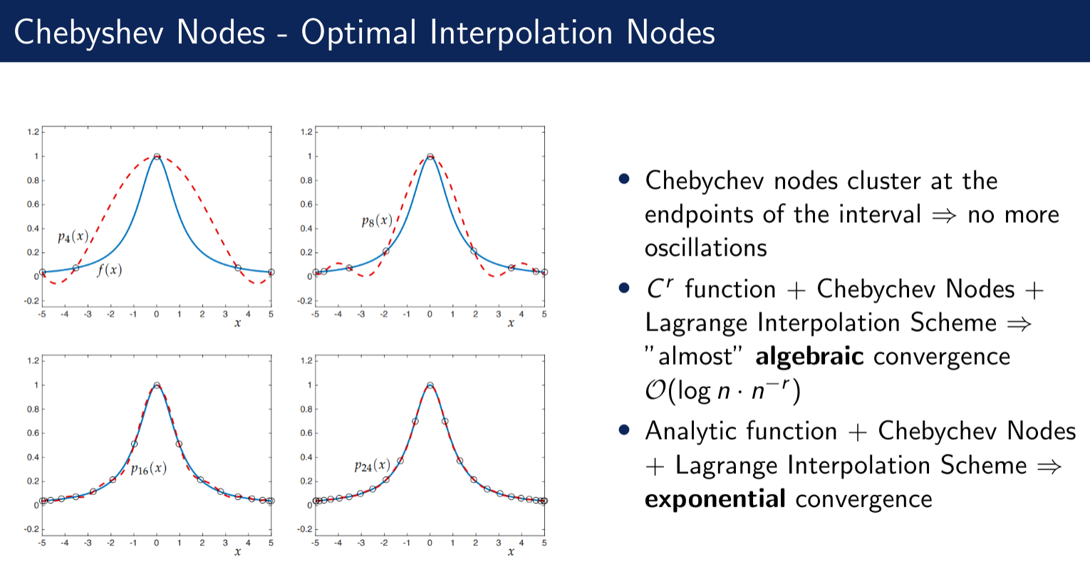
#timestamp 2025-

Gauss QR -> speed of convergence depends on extension on analytic area
Trapezoidal QR -> faster, due to aliasing cancellation for (on strip) (?) analytic periodic functions (+simpler)

#timestamp 2025-11-29

do {
Eigen::Vector4d s = df(x).householderQr().solve(f(x));
x = x - s;
gn_update.push_back(s.norm());
// absolute stopping criteria
} while(gn_update.back() > tol);

Newton-Gauss method, see 8.11)d)

Hiptmair used

s.lpNorm<Eigen::Infinity>();

Infinity-norm stopping is better, because:

it is cheaper to compute,
it treats the largest component directly,
it is less sensitive to cancellation.

He also used

df(x).colPivHouseholderQr().solve(f(x));

The Jacobian in Gauss–Newton can easily become nearly rank-deficient, especially early in the iteration.
Without pivoting, householderQr() may produce an unstable or unusable step. colPivHouseholderQr() safeguards the solve by reordering the columns so that the effective conditioning is improved.

#timestamp 2025-12-05

Explicit Euler Method
- gets inaccurate pretty fast
+ easy to implement

$E (h) = O (h)$ (order 1)

Implicit Euler Method

uses backwards quotient instead of time quotient

- more complicated, because $y_{k + 1}$ on both sides -> non-linear SE at every iteration
- not faster that explicit method (order 1) (?)

$E (h) = O (h)$ (order 1)

Implicit Midpoint Method
- left and right side depend on value of next iterate -> non-linear SE

-> asymptotic of single-step methods can only be controlled by choosing the mesh

$E (h) = O (h^{2})$ (order 2)

Bootstrap method
+ explicit -> linear SE
+ order $p > 2$

Explicit Midpoint Method = Midpoint QR + Explicit Euler
- algebraic cvg, p=2
Explicit Trapezoidal Method = Trapezoidal QR + Explicit Euler
- algebraic cvg, p=2

Explicit Runge-Kutta Single-Step Method