ETH_NumericalMethodsForPDE

links - NumPDE

website: grausam
- local copy: NUMPDE.pdf
script: https://people.math.ethz.ch/~grsam/NUMPDEFL/NUMPDE.pdf
exercises: grausam/NPDEFL_Problems.pdf
- local copy: NPDEFL_Problems.pdf
exercise repository: https://gitlab.math.ethz.ch/ralfh/NPDERepo

useful links

cpp reference: https://en.cppreference.com/
lehrfm: GitHub / doxygen
eigen documentation: https://eigen.tuxfamily.org/

Info

exam
- NumPDE midterm (@2026-04-17)
  - chapter 1+2 (mainly)
- NumPDE endterm (@2026-05-29)
  - chapter Stokes + Navier (?)
practice classes:
- ETH_NumericalMethodsForPDE_Übungen

Info

HPK D 3 (13:45, Thu) https://polybox.ethz.ch/index.php/s/dM5NqE3wqeWYsNp
CAB G 61 (14:00, Thu) https://polybox.ethz.ch/index.php/s/Xen2eXQaoQd6Css

Hilfsmittel NumericalMethodsForPartialDifferentialEquations

midterm: probably none
endterm: probably none

Exercises

-> FS2026_tasks

Week 1 (16.02.-20.02.): 4 h 45 min

Problem 0-1: Setting up implementation environment for NumPDE course (60 min)
Problem 0-2: Using the GDB Debugger (80 min)
Problem 1-1: Quadratic Functionals (100 min) (c) not sure about sums, (b) solved differently)
Problem 1-3: L-infinity Norms are Bounded by H1-seminorms in 1D (45 min) b) solved with Chat

Week 2 (23.02.-27.02.): 6 h 45 min

Problem 1-10: From Boundary Value Problems to Variational Problems (60 min) c) a bit cryptic
Problem 1-6: heat conduction with non-local boundary conditions (75 min) c) important, applies most of the learned norms/inequalities
Problem 1-8: A coupled reaction-diffusion problem (60 min)
Problem 1-5: A second-order elliptic transmission problem in 1D (110 min) do again tomorrow?
Problem 1-2: Linear functionals on Sobolev spaces (100 min)
- solution for h): 20260226_NumPDE_1.2)h)

Week 3 (02.03.-06.03.): 7 h 5 min

Problem 2-3: Pointwise "Exact" Galerkin Solution (65 min)
Problem 2-1: Properties of Galerkin solutions (45 min) much longer than 45min, c), d) enjoyable
Problem 2-2: Transformation of Galerkin Matrices (120 min) skipped d), copied e)
Problem 2-4: Linear finite elements for two-point boundary value problems (195 min) demanding exercise, took ≅3.5h; didn't understood last part (offset function)

Week 4 (09.03.-13.03.): 5 h 45 min

Problem 2-23: Galerkin Matrices (35 min)
Problem 2-20: DofHandler and Assembly (30 min)
Problem 2-9: Handling degrees of freedom (DOFs) in LEHRFEM++ (140 min) last few subtasks done with LM
Problem 2-8: Introduction to local assembly in LEHRFEM++ (140 min) couldn't implement j) myself

Week 5 (16.03.-20.03.): 7 h 5 min

Problem 2-24: Paramatric FEM: Local Computations (20 min) maybe do again
Problem 2-17: Local Computations for Convection Bilinear Form (90 min) solved in <90min, but didn't understand e) completely
Problem 2-21: Blended Parametric Representation of Curvi-Linear triangles (145 min) f) a bit tricky, but mostly understood
Problem 2-13: Local computations for parametric Lagrangian finite elements (170 min) took ~250min, quite difficult (especially writing the tests); I still don't understand the boundary logic

Week 6 (23.03.-27.03.): 5 h 50 min

Problem 2-22: Constrained Neumann Problem (125 min) a)-f) simple, g) uses summation trick that took me quite some time to understand; overall, took ~90min
Problem 2-18: Nitsche's Method for Elliptic BVPs (225 min) d)e)f) (coding) confusing - couldn't find error - should definitely be solved a 2nd time

Videos

0.0 Welcome and introduction (17min)

week (16.02.-20.02.):

1.2.1 Elastic Membranes (17 min)
1.2.2 Electrostatic Fields (6 min)
1.2.3 Quadratic Minimization Problems (21 min)
1.3 Sobolev spaces (22 min)
1.4 Linear Variational Problems (21 min) didn't quite understand

week (23.02.-27.02.):

1.5 Equilibrium Models: Boundary Value Problems (22 min)
1.6 Diffusion Models: Stationary Heat Conduction (5 min)
1.7 Boundary Conditions (07.35 min)
1.8 Second-Order Elliptic Variational Problems (13 min) even solved question :)
1.9 Essential and Natural Boundary Conditions (18 min)

week (02.03.-06.03):

2.2 Principles of Galerkin Discretization (25 min) review questions for 2.2.3 solved -> review questions for this chapter are important !!
2.3 Case Study: Linear FEMfor Two-Point Boundary Value Problems (24 min)
2.4 Case Study: Triangular Linear FEMin Two Dimensions I (28 min)
2.4 Case Study: Triangular Linear FEMin Two Dimensions II (32 min) confusing

week (09.03.-13.03):

2.5 Building Blocks of General Finite Element Methods (22 min) easy :)
2.6 Lagrangian Finite Element Methods (23 min)
2.7.2 Mesh Information and Mesh Data Structures (21 min) first LehrFM introduction
2.7.4 Assembly Algorithms (26 min)
2.7.5 Local Computations (26 min)
2.7.6 Treatment of Essential Boundary Conditions (21 min)

week (16.03.-20.03):

2.8 Parametric Finite Element Methods I (22 min)
2.8 Parametric Finite Element Methods II (27 min) ??
3.1 Abstract Galerkin Error Estimates (20 min)
3.2 Empirical (Asymptotic) Convergence of Lagrangian FEM (26 min) understandable

week (23.03.-27.03.):

3.3 A Priori (Asymptotic) Finite Element Error Estimates I (10 min)
3.3 A Priori (Asymptotic) Finite Element Error Estimates II (18 min)
3.3 A Priori (Asymptotic) Finite Element Error Estimates III (16 min)
3.4 Elliptic Regularity Theory (11 min)
3.5 Variational Crimes (15 min)
3.8 Validation and Debugging of Finite Element Codes (13 min)

week (30.03.-03.04.):

9.2.1 Heat Equation (10 min)
9.2.2 Heat Equation: Spatial Variational Formulation (8 min)
9.2.3 Stability of Parabolic Evaolution Problems (10 min)
9.2.4 Spatial Semi-Discretization: Method of Lines (6 min)
9.2.7 Timestepping for Method-of-Lines ODE (30 min) rewatch
9.2.8 Fully Discrete Method of Lines: Convergence (18 min) first 6min summary of chapter 9)

week (13.04.-17.04.):

10.1.1 Modeling Fluid Flow (7 min)
10.1.2 Heat Convection and Diffusion (5 min)
10.1.3 Incompressible Fluids (10 min)
10.1.4 Time-Dependent (Transient) Heat Flow in a Fluid (4 min)
10.2.1 Singular Perturbation (16 min)
10.2.2 Upwinding (13 min)
10.2.2.1 Upwind Quadrature (17 min)
10.2.2.2 Stremline Diffusion (19 min)
10.3.1 Method of Lines (13 min)

week (20.04.-24.04.):

12.1 Modeling the Flow of a Viscous Fluid (30 min)
12.2.1 The Stokes Equations: Constrained variational formulation (20 min)
12.2.2 The Stokes Equations: Saddle Point Problem Formulation (55 min)
12.2.3 Stokes System of Partial Differential Equations (15 min)

week (27.04.-01.05.):

12.3.1 Pressure Instability (40 min)
12.3.2 Stable Galerkin Discretization of Stokes Saddle Point Problem (30 min)
12.3.3 Convergence of Stable FEM for Stokes (30 min)
12.3.4 The Taylor-Hood Finite Element Method (15 min)
12.3.5 The Non-Conforming Crouzeix-Raviart FEM (40 min)

week (04.05.-08.05.):

13.1.2 Fields and Integral Forms/Currents (28 min)
13.1.3 Differential Forms (56 min)
13.1.4 Exterior Calculus (70 min)
13.1.5 Sobolev Spaces of Differential Forms (18 min)

week (11.05.-15.05.):

13.2.1 Cochain Calculus (67 min)
13.2.2 Whitney Forms (70 min)
13.3.1 Energies and Linear Material Laws (35 min)
13.3.2.1 Electromagnetic Wave Equations (45 min)
13.3.2.3 Method of lines for Electromagnetic Wave Equations, Timestepping for Semi-Discrete Electromagnetic Wave Equations (45 min)

week (18.05.-22.05.):

13.3.3.1 Magnetostatics: Formulations Based on Scalar Potentials (30 min)
13.3.3.2 Magnetostatics: Vector-Potential-Based Variational Formulations (40 min)
13.3.3.3-13.3.3.4 Saddle-Point Variational Problems, Discrete LBB-Conditions for a-Based Magnetostatics (60 min)

week (25.05.-29.05.): no videos

Q&A

#timestamp 2026-03-20

Galerking Orthogonality (3.1.3.2)

$∥ u - u_{h} ∥_{a}^{2} = a (u - u_{h}, u - u_{h}) = a (u - v_{h}, u - u_{h}) + \underset{= 0}{\underset{⏟}{a (v_{h} - u_{h}, u - u_{h})}} \forall v_{h} \in V_{0, h}$

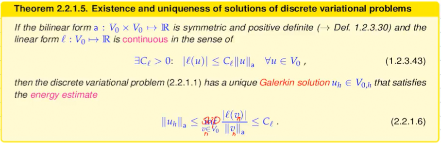
bilinear form is coercive

continuity / boundedness: $| a (u, v) | \leq C ∥ u ∥_{v} ∥ v ∥_{v}$
coercivity: $γ ∥ u ∥_{v}^{2} \leq | a (u, u) |$

from this comes the Poincare inequality and uniform positive definite property

In contrast to Cea's Lemma, coercivity does not depend on the energy norm

∥ \cdot ∥_{a}

Tldr: strong to weak

$- (\partial_{1} \partial_{1} u + \partial_{1} \partial_{2} u + \partial_{2} \partial_{2} u) + ∥ x ∥^{2} u = 0 \in Ω, u = 1 \in \partial Ω$

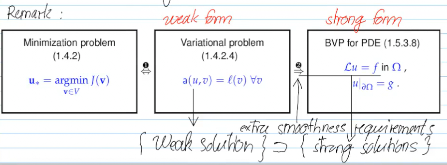
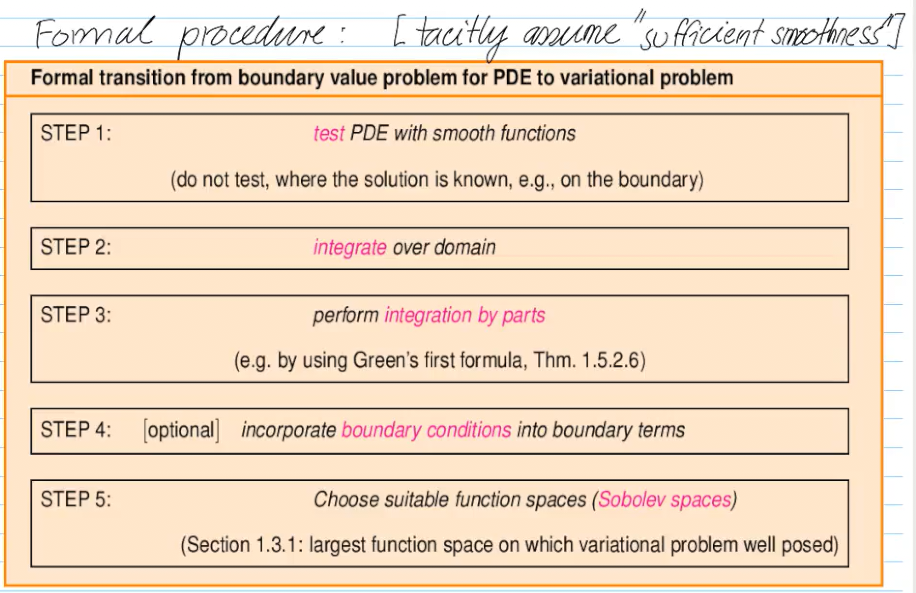
(simplify strong form, then) convert to weak form

\begin{array}{r} - div ([\begin{array}{c} 1 & \frac{1}{2} \\ \frac{1}{2} & 1 \end{array}] \nabla u) + ∥ x ∥^{2} u = 0 ⟹ - div (A \nabla u) + β u = 0 \\ \int - div (A \nabla u) v + β u v d x = 0 \end{array}

choose suitable test function

e.g. $v \in C_{0}^{\infty} \subset H^{1} (Ω)$

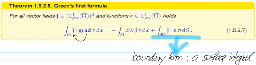
IBP (use Green's formula)

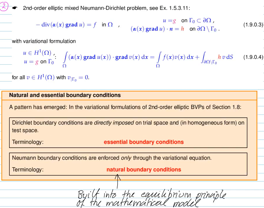
\int_{Ω} A \nabla u \nabla v + β u v d v - \underset{0 by b.c.}{\underset{⏟}{\int_{\partial Ω} A \nabla u \cdot n v d l}} = 0

Incorporate b.c. (if needed)

for Dirichlet (essential) -> nothing to do

choose suitable fct. space

minimal suitable fct. space (often $H^{1}$ )
here, we need at list one derivative for $\nabla u$

\int A \nabla u \nabla v + β u v d x = 0 \forall v \in H_{0}^{1} (Ω)

Vorlesung

1. Second-Order Scalar Elliptic Boundary Value Problems

Video 1.2.1: Elastic Membranes

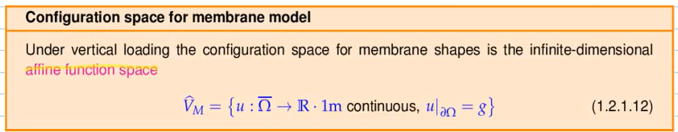
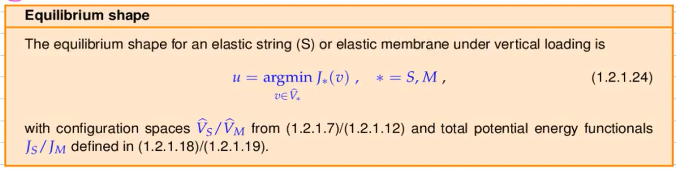
Goal: compute shape of string (1D)/membrane (2D) under vertical loading

Notion 1.2.1.1. Configuration space

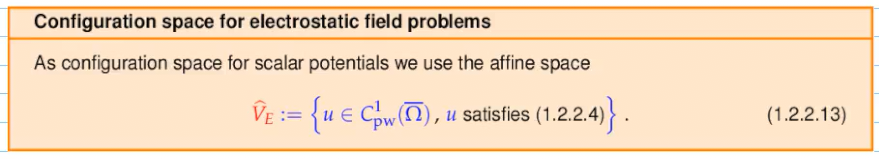
The configuration space of a mathematical model is a set, each of whose elements completely describe all relevant aspects of a state of the modeled physical system.

string must be continuous $⟺$ string not ripped apart
b.c.: u(a),u(b) given

Pasted image 20260216223006.png
Pasted image 20260216223153.png
Pasted image 20260216223325.png
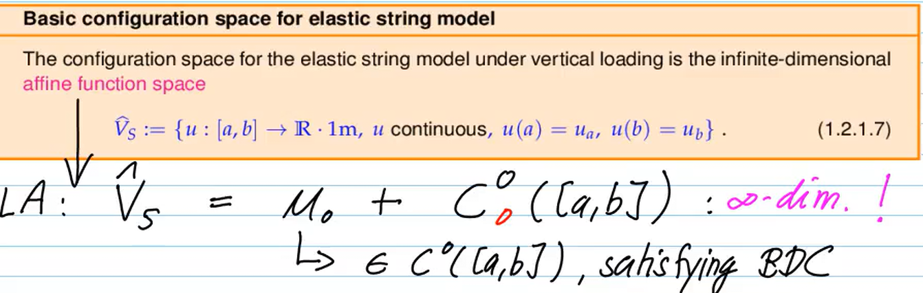
-> but need formula for potential energy
Pasted image 20260216223452.png

Video 1.2.2 Eloectrostatic Fields (6min)

Pasted image 20260217102058.png
Pasted image 20260217102244.png
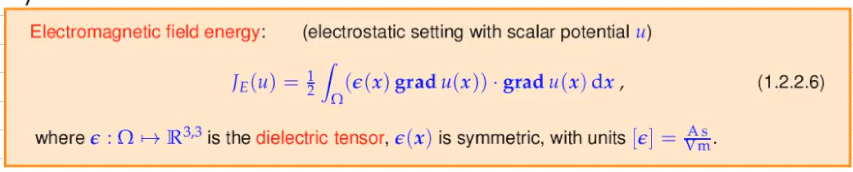
Note: $\hat{V} \subset C^{0} (\overset{―}{Ω})$

Equilibrium condition for electrostatics

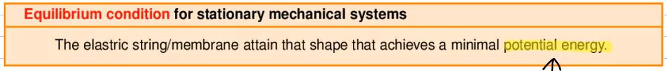
The physical field will attain minimal electromagnetic field energy (1.2.2.16)

u_{*} = \underset{u \in {\hat{V}}_{E}}{argmin} J_{E} (u) .

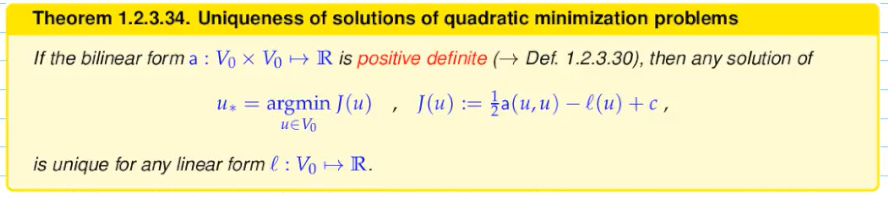
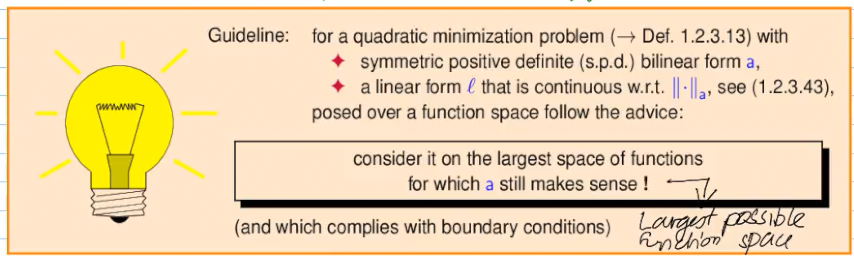
Video 1.2.3 Quadratic Minimization Problems (21 min)

Pasted image 20260217102711.png

Definition 1.2.3.13. Quadratic minimization problem

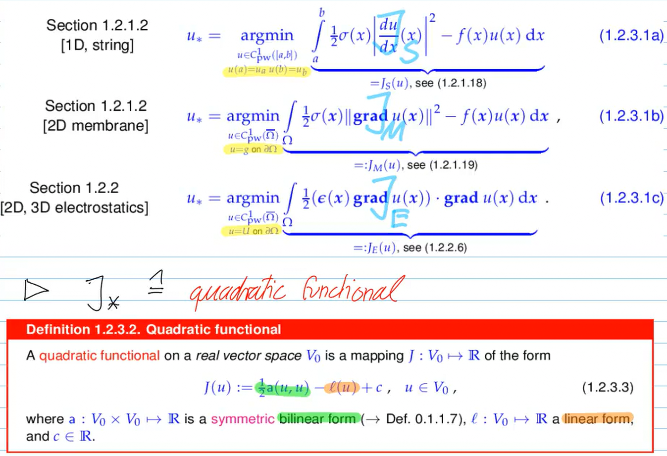
A minimization problem

w_{*} = \underset{w \in V_{0}}{argmin} J (w)

is called a quadratic minimization problem, if $J$ is a =quadratic functional on a real vector space $V_{0}$ .

extension to affine space:

\hat{V} = \underset{"offset function"}{\underset{⏟}{μ_{0}}} + V_{0} \subset V

Pasted image 20260217103305.png
Pasted image 20260217103546.png
Recall from LA:

A = A^{⊤} s.p.d ⟹ (\vec{μ}, \vec{η}) \to {\vec{μ}}^{⊤} A \vec{η} \hat{=} inner product

Pasted image 20260217104011.png
Pasted image 20260217104355.png

Tldr

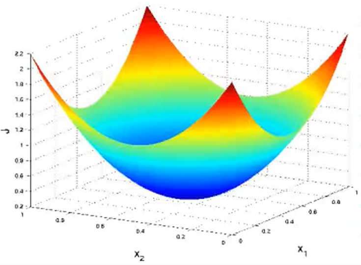
we are trying to find the most stable/lowest energy state of the system. The idea is to find a general formula for the structurally similar string/membrane/electricity problem, which can be described by a Quadratic functional:

J (v) = \underset{internal energy}{\underset{⏟}{\frac{1}{2} a (v, v)}} - \underset{external load}{\underset{⏟}{l (v)}} + c = \frac{1}{2} x^{⊤} A x - b^{⊤} x + c (a bilinear + symmetric, l linear)

However, we can only solve the problem if the energy formula has a minimum (imagine the energy formula as a paraboloid "bowl"):
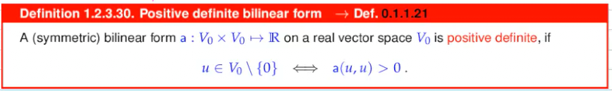
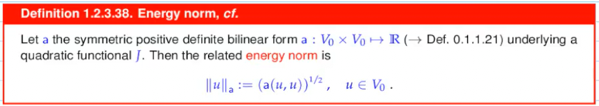
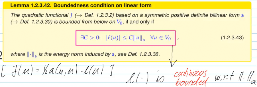
Pasted image 20260217110348.png|300
Thus, for $\exists$ of solution, the problem must fulfill:

$a (v, v) > 0 \forall v \neq 0$ -> bilinear form must be at least semi-positive definite
$| l (v) | \leq C | | v | |_{a}$ , where $| | v | |_{a} = \sqrt{a (v, v)}$ energy norm. -> linear form $l (v)$ must be bounded/continuous with respect to energy norm. This ensures the "load" isn't so strong that it rips the system apart.

#todo add some integrals to the tldr

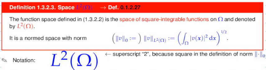
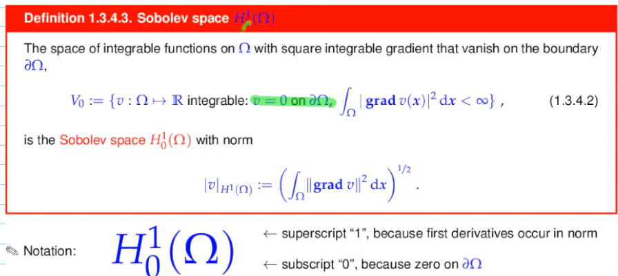
Video 1.3 Sobolev spaces (22 min)

have a bad reputation as having a useless mathematical sophistication

Pasted image 20260217113247.png
choose

V_{0} := {functions v on Ω : a (v, v) < \infty}

=> energy space generated by $a (\cdot, \cdot)$
Pasted image 20260217113422.png
Pasted image 20260217113818.png
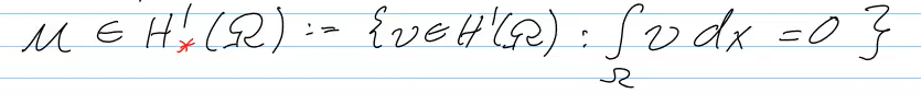
in contrast to $L^{2}$ -Space, here the boundary conditions are not dropped; the reason for this are the norms:
Pasted image 20260217114017.png
Sobolev space without boundary conditions:
Pasted image 20260217114124.png
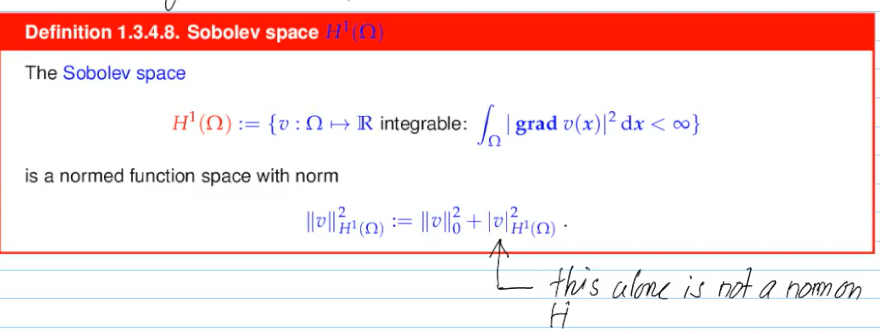
the $L^{2}$ can be bounded by the size of the domain and the energy norm:

Theorem 1.3.4.17: First Poincaré-Friedrichs inequality

If $Ω \subset R^{d}$ , $d \in N$ , is bounded, then

∥ u ∥_{0} \leq diam (Ω) ∥ grad u ∥_{0} \forall u \in H_{0}^{1} (Ω) .

$⟹ | ℓ (v) | \leq \underset{C}{\underset{⏟}{∥ f ∥_{0} diam (Ω)}} ∥ v ∥_{a} \forall v \in H_{0}^{1} (Ω)$

Pasted image 20260217114451.png

How to "work with" Sobolev spaces

Most concrete results about Sobolev spaces boil down to relationships between their norms. The spaces themselves remain intangible, but the norms are very concrete and can be computed and manipulated as demonstrated above.

Tip

Do not be afraid of Sobolev spaces!
It is only the norms that matter for us, the 'spaces' are irrelevant!

Corollary 1.3.4.26.

H^{1}

-norm of piecewise smooth functions

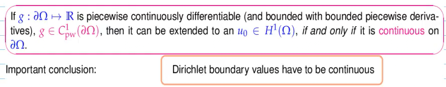
Under the assumptions of Thm. 1.3.4.23 we have for a continuous, piecewise smooth function $u \in C^{0} (Ω)$

{| u |}_{H^{1} (Ω)}^{2} = | u |_{H^{1} (Ω_{1})}^{2} + | u |_{H^{1} (Ω_{2})}^{2} = \int_{Ω_{1}} | grad u (x) |^{2} d x + \int_{Ω_{2}} | grad u (x) |^{2} d x .

If $u \in C^{0} (Ω) \Rightarrow$ compute $H^{1}$ -norm piecewise

Tldr

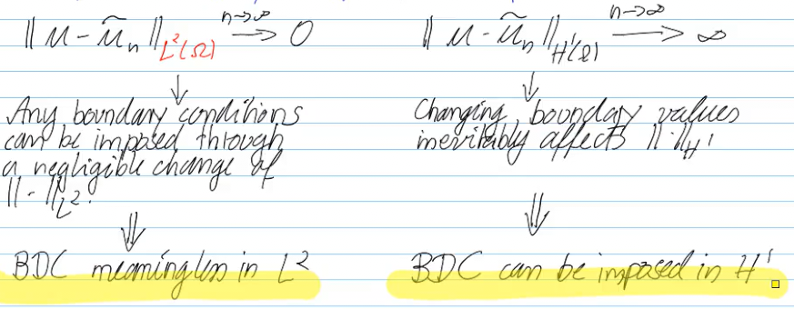
$L^{2}$ space - space of all functions where $\int f^{2} < \infty$ . Here, b.c. are meaningless, since changing the function at a single point costs zero energy
$H^{1}$ space - "energy space" for membranes; includes functions where derivatives are square-integrable. Unlike $L^{2}$ , the b.c. cannot be ignored, since changing a point blows up the derivative
$H_{0}^{1}$ -space - $H^{1}$ with zero b.c.
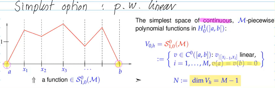
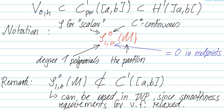
- one can think of $H^{1}$ as the space of peicewise smooth, globally continuous functions

Tldr

Functions of an $L^{2}$ space are square-integrable on $Ω$ :

\int_{Ω} | u (x) |^{2} d x < \infty

Functions of the $H^{1}$ space are in $L^{2}$ , too. Additionally, the first (hence ^1) derivative is in $L^{2}$ , too:

H^{1} (Ω) = {u \in L^{2} (Ω) | \nabla u \in L^{2} (Ω)}

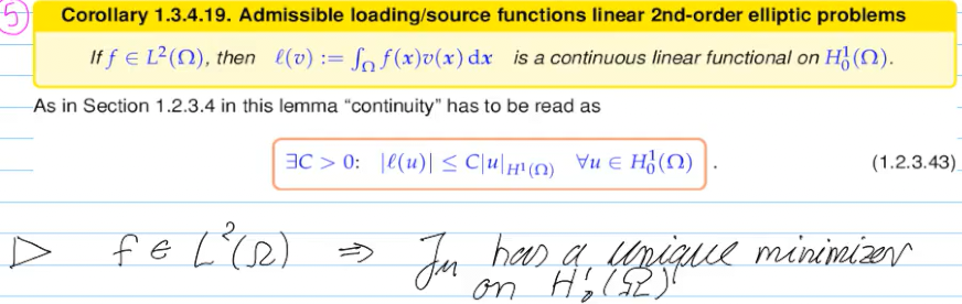
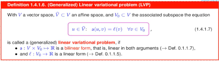
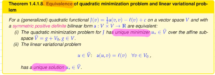
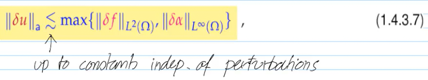
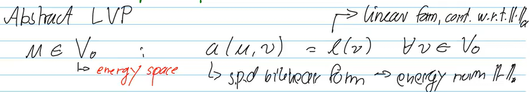
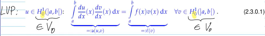
Note that $H^{1}$ functions do not need to be in $C^{1}$ or even $C^{0}$ ! A counterexample is

u (x, y) = {\begin{cases} 0, & x \leq \frac{1}{2} \\ 1, & x > \frac{1}{2} \end{cases} in Ω = [0, 1]^{2}

Video 1.4 Linear Variational Problems (21 min)

Pasted image 20260219081701.png
Pasted image 20260219082140.png
Pasted image 20260219082308.png
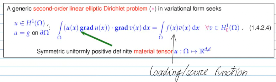
Poincare-friedrich?
Pasted image 20260219082838.png

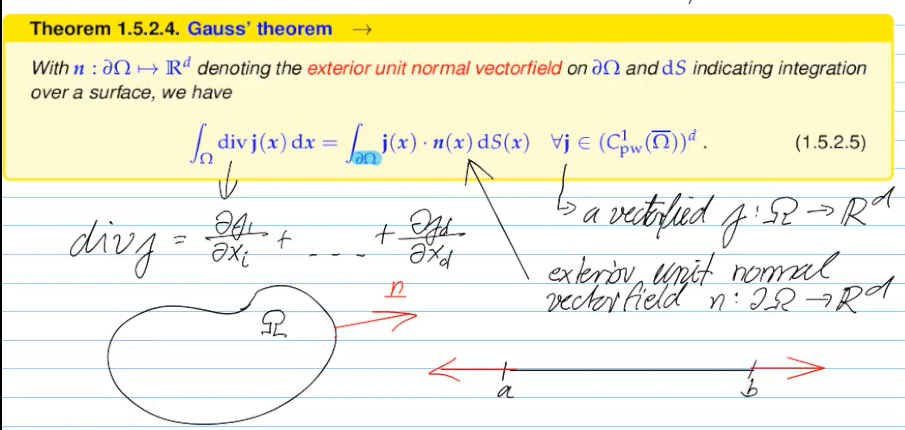
Video 1.5 Equilibrium Models: Boundary Value Problems (22 min)

Pasted image 20260224174310.png
Pasted image 20260224175303.png
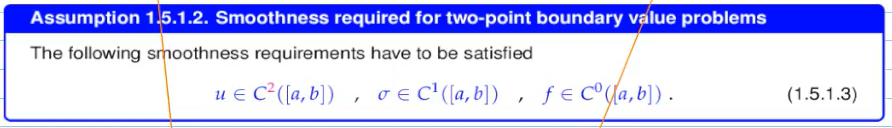
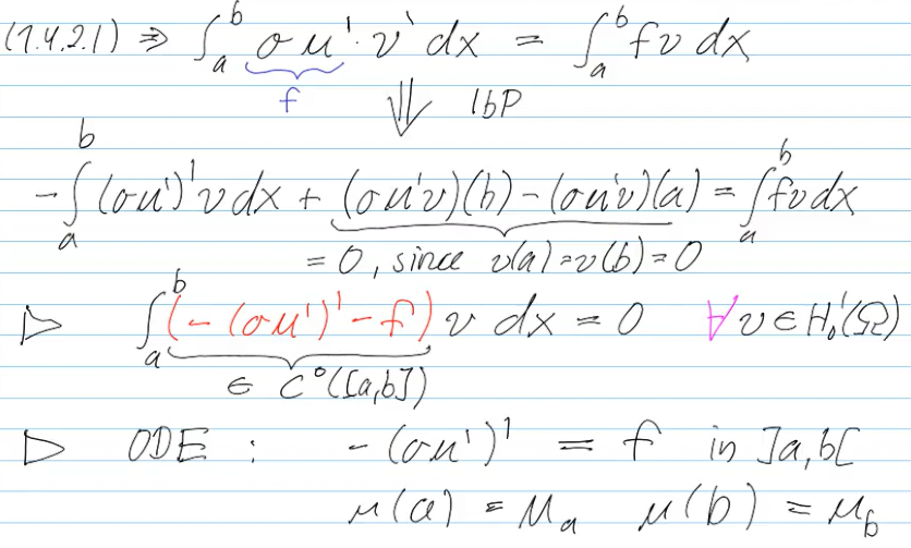
=> 2-pt BVP (a Dirichlet problem) in strong form (vs. "weak form" = LVP)

Pasted image 20260224175546.png
Pasted image 20260224175607.png

Lemma 1.5.3.4: Fundamental lemma of calculus of variations in higher dimensions

If $f \in L^{2} (Ω)$ satisfies

\int_{Ω} f (x) v (x) d x = 0 \forall v \in C_{0}^{\infty} (Ω),

then $f \equiv 0$ can be concluded.

Pasted image 20260224180021.png
Pasted image 20260224180509.png

Video 1.6 Diffusion Models: Stationary Heat Conduction (5 min)

Pasted image 20260224182905.png
Pasted image 20260224183014.png
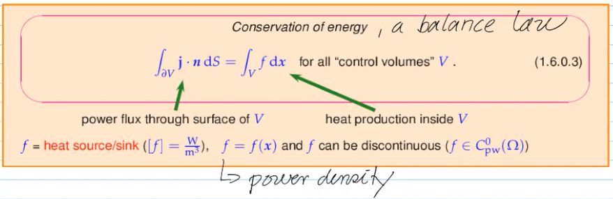
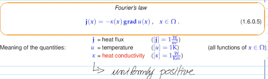
by combining those two using Gauss theorem, we get:
Pasted image 20260224183120.png
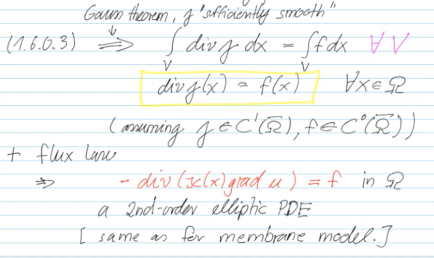
=> we reach at the same PDE as for the membrane model

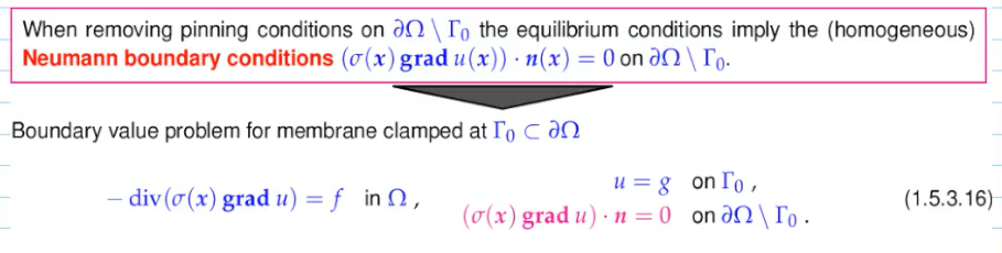
Video 1.7 Boundary Conditions (07.35 min)

Pasted image 20260224183718.png
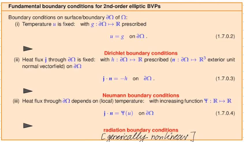
example of a mixed BVP:
Pasted image 20260224184006.png

Boundary conditions for second-order elliptic BVPs

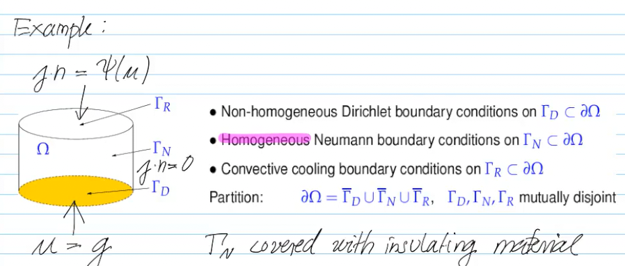
For second order elliptic boundary value problems exactly one boundary condition is needed on every part of $\partial Ω$ .

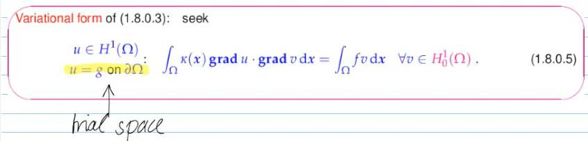
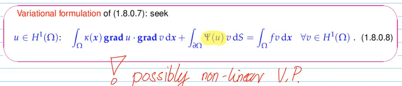
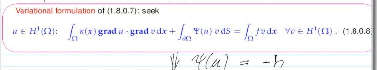
Video 1.8 Second-Order Elliptic Variational Problems (13 min)

Pasted image 20260224190120.png
for Dirichlet BVP:
Pasted image 20260224213109.png
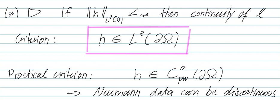
for Radiation BVP:
Pasted image 20260224213302.png
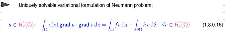
for Neumann BVP:
Pasted image 20260224214942.png
Pasted image 20260224215319.png
Pasted image 20260224215332.png

Theorem 1.8.0.20: Second Poincaré-Friedrichs inequality

If $Ω \subset R^{d}$ , $d \in N$ , is bounded, then

\exists C = C (Ω) > 0 : ∥ u ∥_{0} \leq C diam (Ω) ∥ grad u ∥_{0} \forall u \in H_{*}^{1} (Ω) .

Video 1.9 Essential and Natural Boundary Conditions (18 min)

summary of 1.4 - 1.9:
Pasted image 20260225081041.png
Pasted image 20260225081059.png
Pasted image 20260225081424.png
Pasted image 20260225082319.png
Pasted image 20260225082332.png

Tldr

For a summary of this week, see the notes from the exercise session:
-> ETH_NumericalMethodsForPDE_Übungen#^75b794

2. Finite Element Methods (FEM)

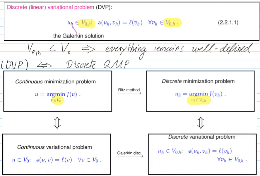
Video 2.2 Principles of Galerkin Discretization (25 min)

graph LR
	A[Variational boundary
value problems] -- discretization --> B["System of a finite number of equations for (real) unknowns"]

Pasted image 20260301110814.png

garlekin discretization in two steps:

$V_{0} \to V_{0, h} \subset V, \dim V_{0, h} < \infty$

Galerkin discretization (step 1)

Replace the infinite-dimensional function space $V_{0}$ in the linear variational problem (2.2.0.2) with a finite-dimensional subspace $V_{0, h} \subset V_{0}$ .

-> "h" $\hat{=}$ tag for s.th. finite

Pasted image 20260301111127.png
Pasted image 20260301111209.png

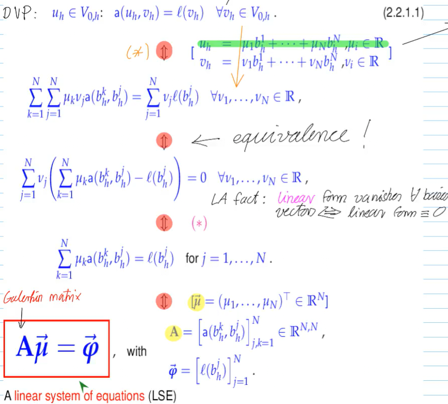
Choose basis, then plug basis expansions int DVP, and use (bi-linearity)

Pasted image 20260301111355.png
Pasted image 20260301111722.png|697

Theorem 2.2.2.7: Independence of Galerkin solution of choice of basis

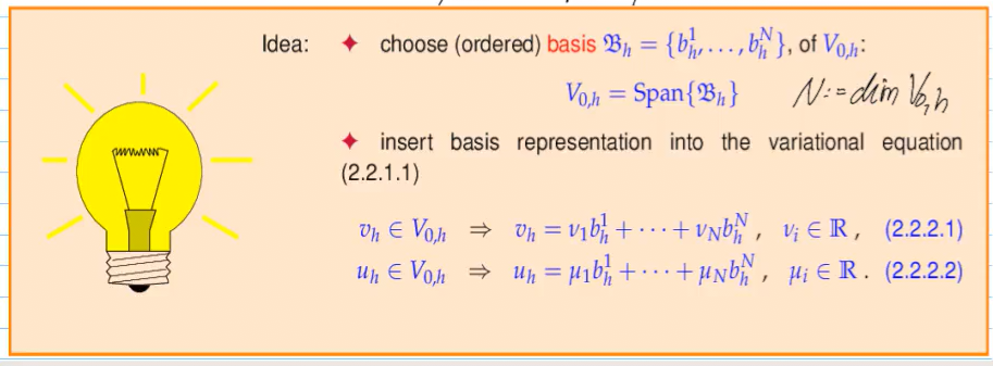
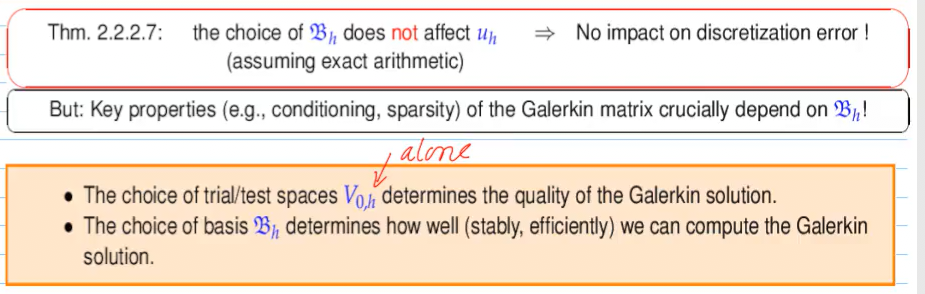
The choice of the basis $B_{h}$ has no impact on the (set of) Galerkin solutions $u_{h}$ of (2.2.1.1).

Pasted image 20260301111839.png
Pasted image 20260301112119.png

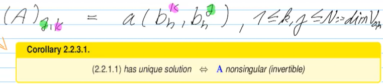
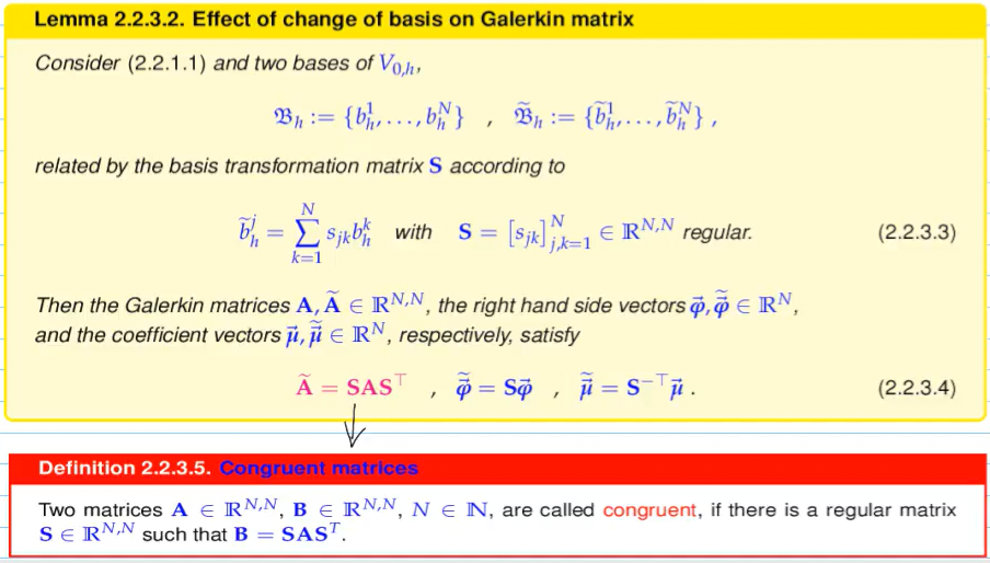
Properties all Garlekin matrices for a DVP (all matrices from a congruence clas) share:

regularity (invertibility)
symmetry
pos.dev.

Garleking pos. dev / symm. ⟺ a (\cdot, \cdot) s.p.d on V_{0, h}

Pasted image 20260301112433.png

Video 2.3 Case Study: Linear FEMfor Two-Point Boundary Value Problems (24 min)

u^{″} = f in [a, b] u (a) = u (b) = 0

NOTE: $f \in L^{2} (Ω)$ is given inprocedural form, $f \in C^{0} ([a, b])$
Pasted image 20260301112821.png

Idea underlying the finite element method: approximate $u$ by means of continuous, piecewise polynomial functions on a mesh:

Pasted image 20260301113228.png
Pasted image 20260301113412.png
Pasted image 20260301114959.png

Video 2.4 Case Study: Triangular Linear FEMin Two Dimensions I (28 min)

In 1D, we partition the domain $Ω$ into an 1D Mesh
In 2D, we use triangulation

Pasted image 20260301182551.png

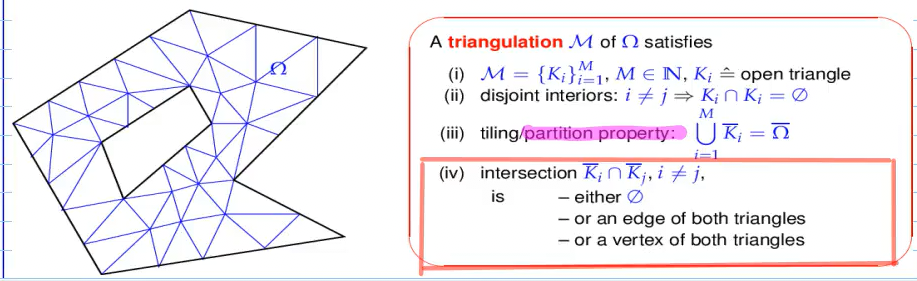
1. means: no hanging nodes (nodes that are on the edge of another triangle)

Pasted image 20260301183038.png

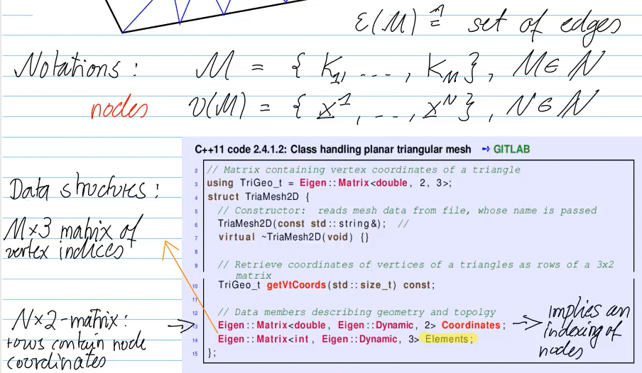
$ϵ (M) =$ set of edges
$M = {K_{1}, \dots, K_{M}}, M \in N$
$v (M) = {{\vec{x}}^{1}, \dots, {\vec{x}}^{N}}, N \in N$

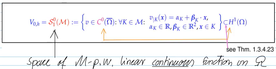
test space in 2 (space of M-p.w. linear continuous function on $Ω$ ):
Pasted image 20260301183355.png

tent function alternative in 2D:
Pasted image 20260301184029.png

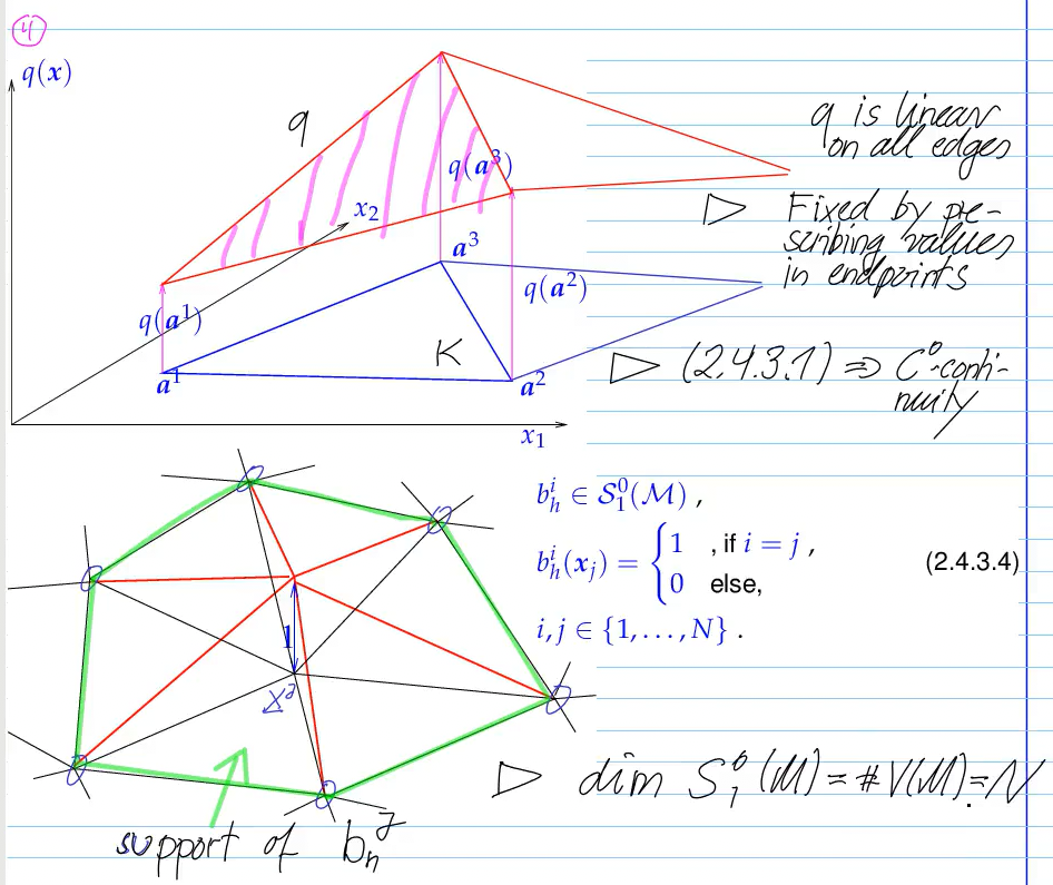
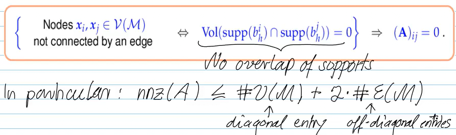
In 2D, the Galerking matrix does not have a nice structure like in 1D; however, it is still sparse, since nodes unconnected by edges result in a 0 in the Matrix:
Pasted image 20260301184700.png

Video 2.4 Case Study: Triangular Linear FEMin Two Dimensions II (32 min)

Galerkin discretization based on a nodal basis of tent functions and a triangular mesh:
Pasted image 20260301203218.png
Pasted image 20260301203646.png
there are two approaches to creating the Galerkin-matrix:

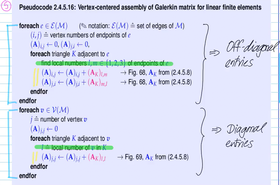
assemble matrix from all vertices

Problems:

Edges not available in data structure (see first 2.4 video)
Triangles adjacent to nodes not available

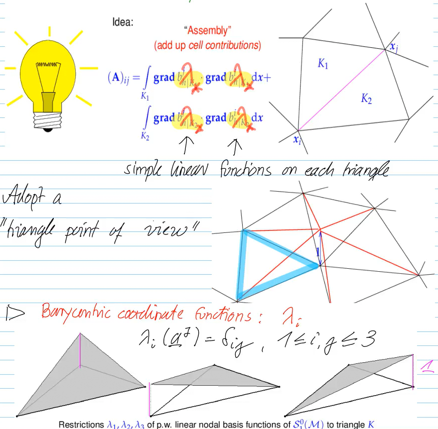
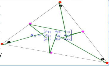
In my opinion, it is not fair to compare it with the cell-oriented approach, when the data class is also cell-oriented

cell-oriented approach, by "distribute & add"

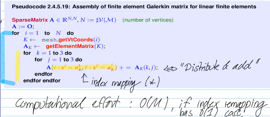
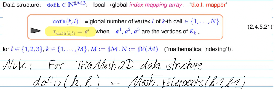
for finite-element algorithms, always do it cell-oriented

Pasted image 20260301205155.png
dof: degrees of freedom
Pasted image 20260301205231.png

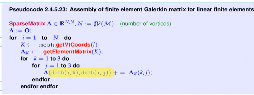
now, we assemble everything:
Pasted image 20260301205651.png
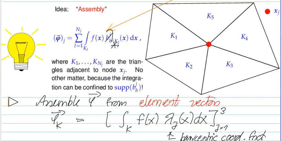
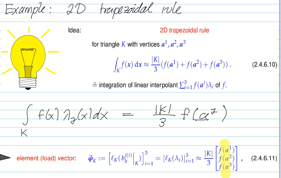
for the RHS, we can compute the integral using composite trapezoidal rule (we are working with triangles anyways):
Pasted image 20260301205803.png

Tldr

We are trying to get variational problems from infinite-dimensional function spaces to something discrete by

choosing a finite-dimensional subspace $V_{0, h} \subset V_{0}$ , where the bilinear and linear form $a (\cdot, \cdot), l (\cdot)$ remain well-defined
choosing an ordered basis ${b_{1}, \dots, b_{N}}$ for the subspace $V_{0, h}, \dim (V_{0, h}) = N$ , and using the basis to convert problem into a linear system

In those two steps, the problem can be transformed into a LSE

A μ = ϕ

Tldr - Step 1

In the first step of the discretization, our goal is to replace space $V_{0}, \dim (V_{0}) = \infty$ with finite $V_{0, h} \subset V_{0}$ . The space should preserve the bilinear form $a (\cdot, \cdot)$ and linear form $l (\cdot)$ . The new problem is:

find u_{h} \in V_{0, h} s.t. a (u_{h}, v_{h}) = l (v_{h}) \forall v_{h} \in V_{0, h}

define Mesh $M$ . Normally, we use triangulation - pay attention that the mesh does not have "hanging nodes" (2.4.1)
choose a "building block" function to use for each cell. Normally, pecewise linear functions are used, evtl. quadratic or cubic polynomials

ensure $C^{0}$ -> do not use piecewise constants, since then $V_{0, h} ⊄ V_{0}$ , e.g. if $V_{0} = H^{1}$

incoroporate boundary conditions, in case of Dirichlet by discarding any basis functions with nodes on the boundary

Tldr - Step 2

4. choose a basis $B_{h} = {b_{1}^{h}, \dots, b_{N}^{h}}$ , then write every $v_{h} \in V_{0, h}$ as linear combination of basis functions:

u_{h} = \sum_{j = 1}^{N} μ_{j} b_{j}^{h}, v_{h} = \sum_{i = 1}^{N} ν_{i} b_{i}^{h}

convert to a linear system by exploiting bilinearity of $a (\cdot, \cdot)$ and linearity of $l (\cdot)$ :

\sum_{j = 1}^{N} μ_{j} a (b_{j}^{h}, b_{i}^{h}) = l (b_{i}^{h}) for i = 1, \dots, N

⟺ A μ = ϕ

$A$ : Galerkin/stiffness matrix, $A_{i j} = a (b_{j}^{h}, b_{i}^{h})$ , how basis functions interact through the bilinear form
$ϕ$ : load vector, $ϕ_{i} = l (b_{i}^{h})$
$μ$ : solution vector; the final Galerkin solution $u_{h} = \sum b_{i}^{h} \cdot μ_{i}$ (basis, weighted by solution vector)

Basis choice

no impact on Galerking solution; however:
basis functions with small local support (e.g. tent function) results in a sparse matrix -> desired outcome
basis choice determines condition number of matrix -> sensitivity to rounding errors

Video 2.5 Building Blocks of General Finite Element Methods (22 min)

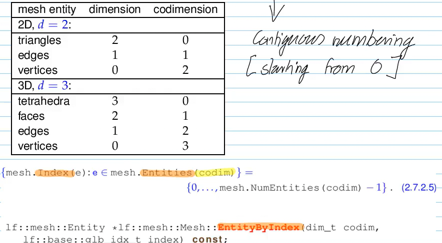
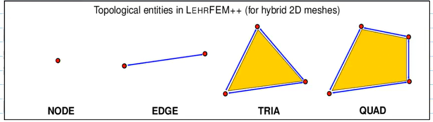
meshes
2D: {cells, edges, nodes}=(mesh/geometric) entities

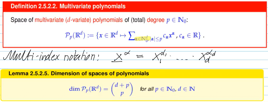
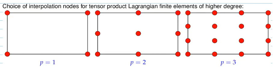
polynomials
Pasted image 20260306093818.png
1st option: e.g.

p = 2 : P_{2} (R^{2}) = span {1, x, y, x^{2}, x y, y^{2}}

Definition 2.5.2.7: Tensor product polynomials

Space of tensor product polynomials of degree $p \in N$ in each coordinate direction

Q_{p} (R^{d}) := {x \mapsto \sum_{ℓ_{1} = 0}^{p} \dots \sum_{ℓ_{d} = 0}^{p} c_{ℓ_{1}, \dots, ℓ_{d}} x_{1}^{ℓ_{1}} \dots x_{d}^{ℓ_{d}}, c_{ℓ_{1}, \dots, ℓ_{d}} \in R}

= Span {x \mapsto p_{1} (x_{1}) \dots p_{d} (x_{d}), p_{i} \in P_{p} (R), i = 1, \dots, d} .

Lemma 2.5.2.8: Dimension of spaces of tensor product polynomials

$\dim Q_{p} (R^{d}) = (p + 1)^{d} for all p \in N_{0}, d \in N$

2nd option: e.g.

Q_{2} (R^{2}) = span {\begin{matrix} 1, x, x^{2} \\ y, y x, y x^{2} \\ y^{2}, y^{2} x, y^{2} x^{2} \end{matrix}}

basis functions (also called global shape functions (GSF), degrees of freedom)

Locally supported basis functions

Third main ingredient of FEM: locally supported basis functions (see Section 2.2 for role of bases in Galerkin discretization)

Basis functions $b_{h}^{1}, \dots, b_{h}^{N}$ for a finite element trial/test space $V_{0, h}$ built on a mesh $M$ must satisfy:

( $B_{1}$ ) $B_{h} := {b_{h}^{1}, \dots, b_{h}^{N}}$ is basis of $V_{0, h} ⟹ N = \dim V_{0, h}$ ,
( $B_{2}$ ) each $b_{h}^{i}$ is associated with a single geometric entity (cell/edge/face/vertex) of $M$ ,
( $B_{3}$ ) $supp (b_{h}^{i}) = ⋃ {\overset{―}{K} : K \in M, p \subset \overset{―}{K}}$ , if $b_{h}^{i}$ associated with cell/edge/face/vertex $p$ .

we want local support:

if $supp (b_{h}^{i})$ , $supp (b_{h}^{j})$ don't overlap, entries in Galerkin matrix $(A)_{i j} = 0$ => sparse matrix

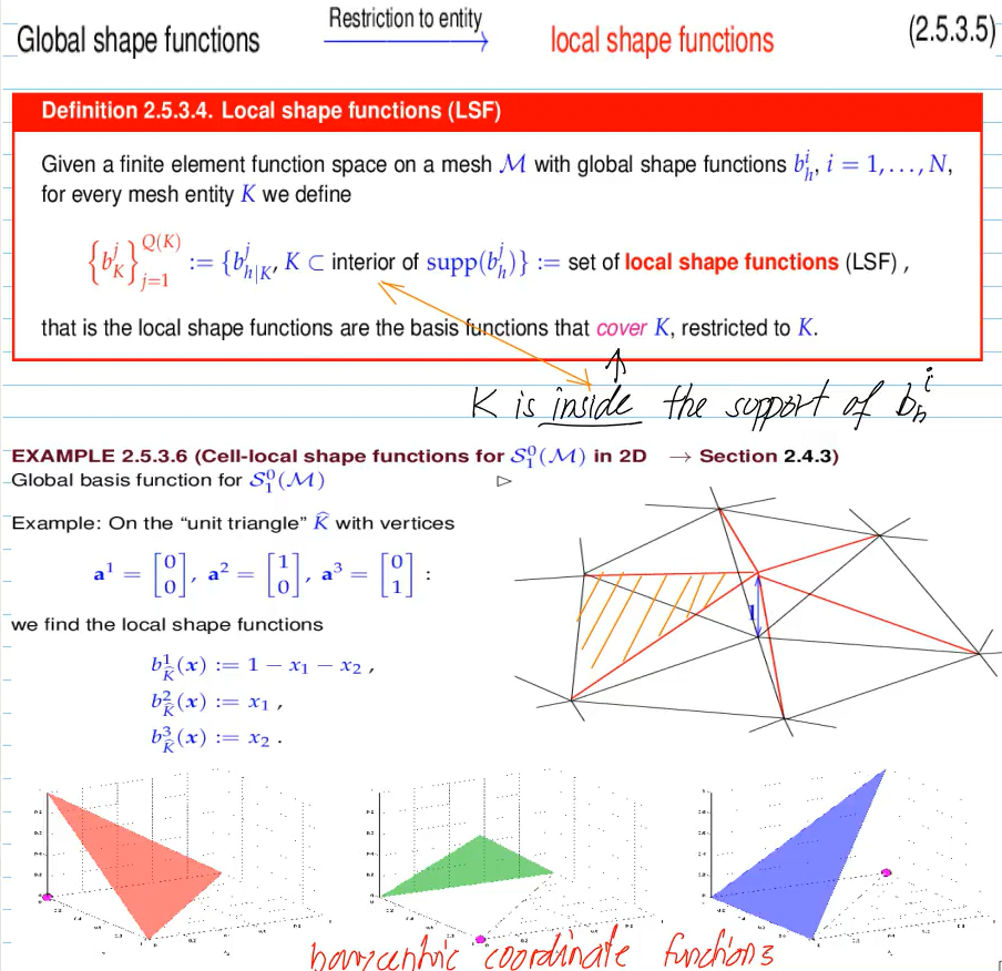
generalization of barycentric coordinate functions:
Pasted image 20260306094819.png

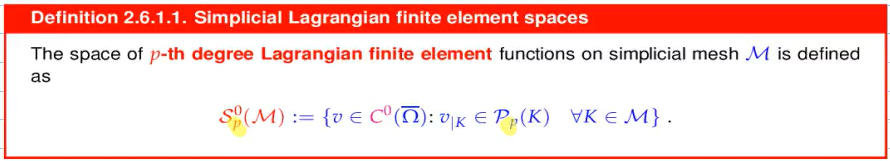
Video 2.6 Lagrangian Finite Element Methods (23 min)

Pasted image 20260310115750.png
one triangle, with Kardinal property:
Pasted image 20260310115836.png
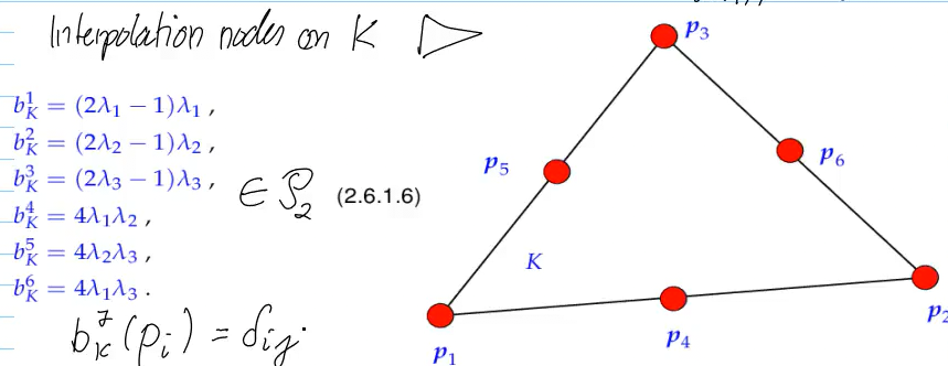
gluing triangles (interpolation nodes):
Pasted image 20260310115922.png
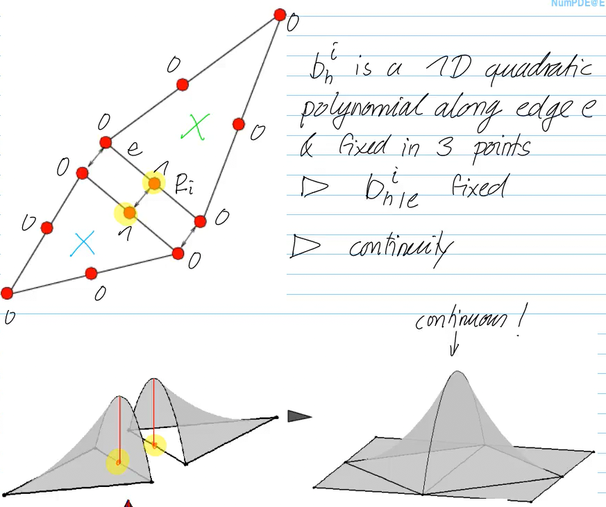
-> globally continuous piecewise function

for more dimensions, we "subdivide"; then, we might also have interpolation nodes inside the shape
Pasted image 20260310120326.png
for hybrid mesh:
Pasted image 20260310120410.png
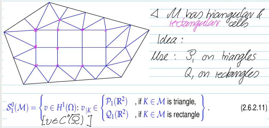
works, becuase functions $\in Q_{1} / P_{1}$ are all linear when restricted to straigt edge (which we have)

works for any degree!

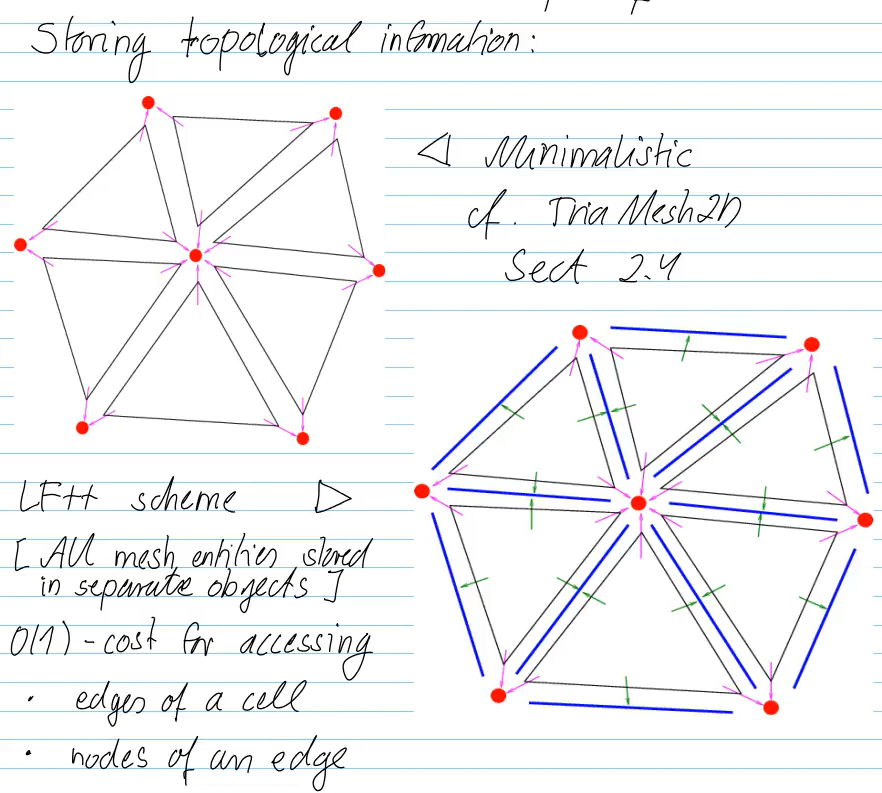
Video 2.7.2 Mesh Information and Mesh Data Structures (21 min)

problems with FEM:
Pasted image 20260310121851.png

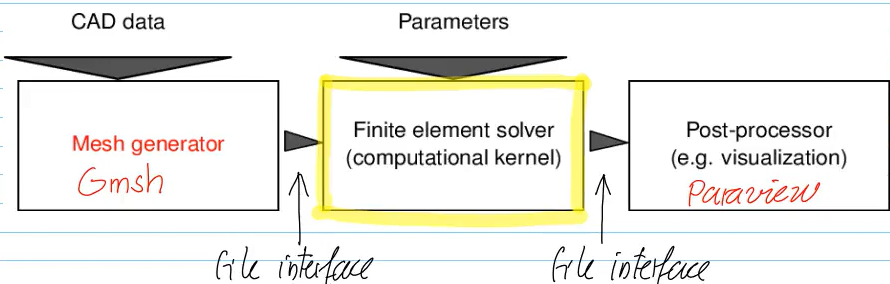
// factory object creates mesg entities auto of 2D mesh data structure from information contained in mesh_file
auto factory = std::make_unique<lf::mesg::hybrid2d::MeshFactory>(2);
lf::io::GmshReader readermove(factory), mesh_file.string();

we need

container (tranversal + ordering/indexing of entities)
topology (incidence/adjecency)
geometry (node locations, entity shapes)

Pasted image 20260310122228.png

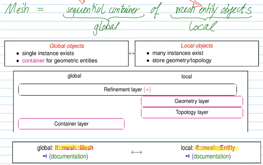
mesh

index access
loops:

for(const lf::mesh::Entity &entity : mesh.Entitiy(codimension));

topology layer
Pasted image 20260310122516.png
Pasted image 20260310122650.png
access:
Pasted image 20260310122726.png

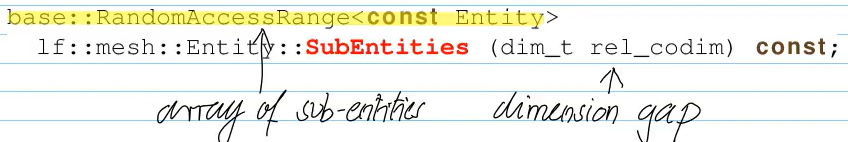
auto sub_entities_range = entity.SubEntities(sub_codimension);
for(const: lf::mesh::Entity &subentity : sub_entities_range)
    mesh.Index(subentity);

geometry layer

geometry object attached for every entity interface

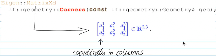
const lf::geometry::Geometry *geo_ptr = entity.Geometry();
Eigen::MatrixXd corners = lf::geometry::Corners(*geo_ptr);

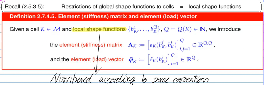
Video 2.7.4 Assembly Algorithms (26 min)

continuation of 2.4

assembly algorithms: building of FE Galerkin amtrix/r.h.s. vector from local contributions

we can split the integrals from the weak form into sums of local contributions (see exercise lession, week3, thu, hongg)
Pasted image 20260310132555.png
Pasted image 20260310133311.png
Pasted image 20260310133322.png
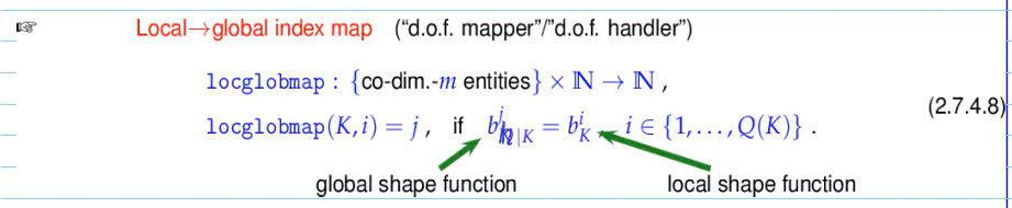
LehrFM numbering rules:
Pasted image 20260310133410.png
Pasted image 20260310133459.png
Pasted image 20260310133904.png

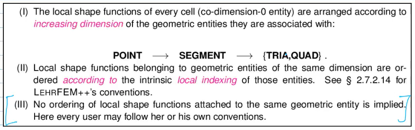
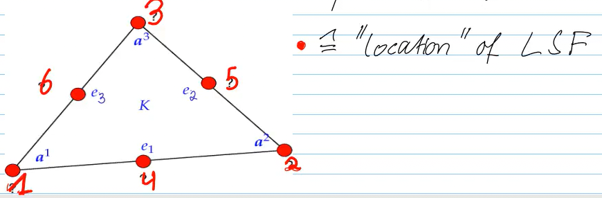
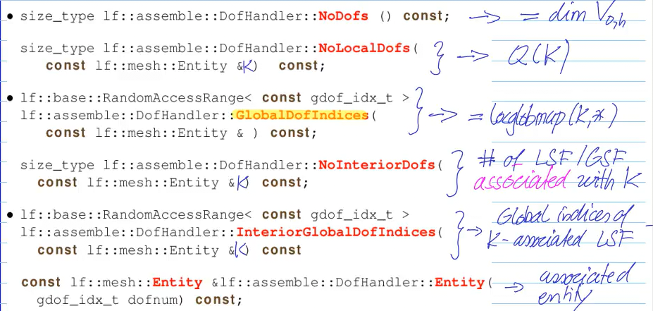
dimension of Space
Number of local Dofs (number of local shape functions)
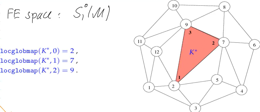
array of locglobmap for all local indices of entity
number of local/global shape functions associatet with entity
global indices of associated local shape functions of indices (not discussed until now)
global index of entity associated with dof

Initalize dynamic Dof Handler:
Pasted image 20260310134015.png
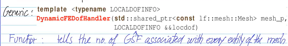
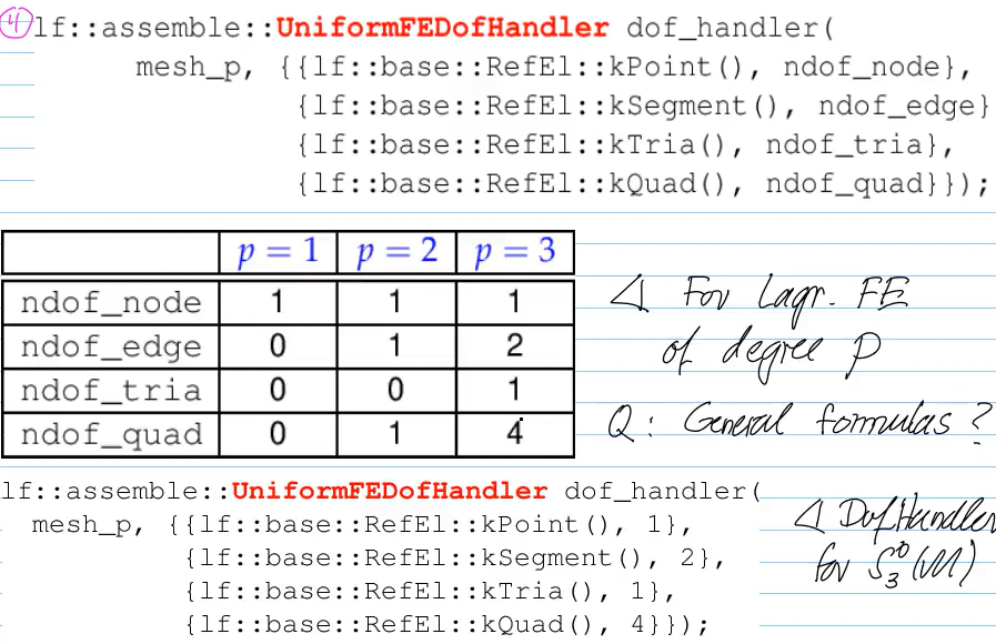
for lagr. FE: uniform no of GSFs associated with entities of same type -> initalization can be simplified:

using dof_map_t = std::map<lf::base::RefEl, base::size_type>;
UniformFEDofHandler(std::shared_ptr<const lf::mesh::Mesh> mesh_p,
                    dof_map_t dofmap);

example:
Pasted image 20260310134056.png
distribute pattern used for assembly

loops over entities + DofHandler queries + local operation

not copied: code 2.7.4.23: Assembly function of LehrFEM++

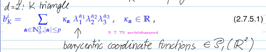
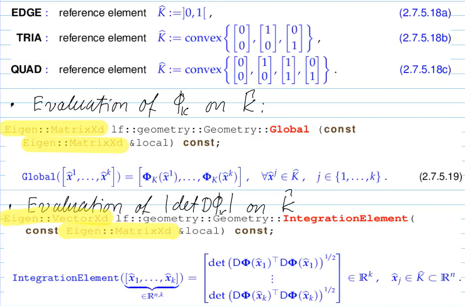
Video 2.7.5 Local Computations (26 min)

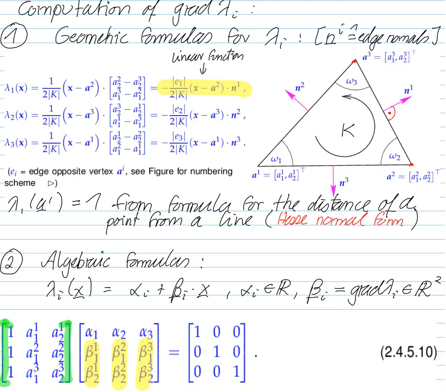
either by analytic computation (only if we have polynomials -> locally constant functions on each cell of the mesh) or

analytic computation:

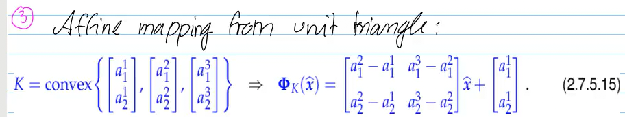
Lemma 2.7.5.5. Integration of powers of barycentric coordinate functions

For any non-degenerate $d$ -simplex $K$ with barycentric coordinate functions $λ_{1}, \dots, λ_{d + 1}$ and exponents $α_{j} \in N, j = 1, \dots, d + 1$ ,

\begin{matrix} (2.7.5.6) & \int_{K} λ_{1}^{α_{1}} \cdot \dots \cdot λ_{d + 1}^{α_{d + 1}} d x = d! | K | \frac{α_{1}! α_{2}! \cdot \dots \cdot α_{d + 1}!}{(α_{1} + α_{2} + \dots + α_{d + 1} + d)!} \forall α \in N_{0}^{d + 1} . \end{matrix}

$↪$ depends only on area of $K$

e.g.
Pasted image 20260310135246.png
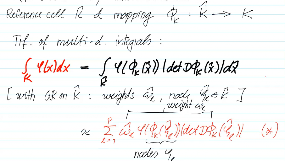
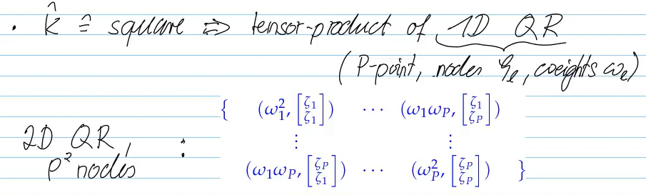
local quadrature

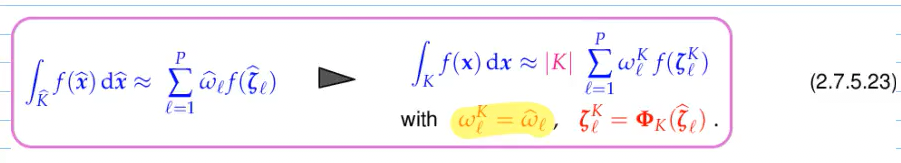
in 1D: affine mapping $[a, b] \to [- 1, 1]$ + transformation formula for integrals
local quadrature rules used in finite element methods are botained by transformation from (a few) local quadrature rules defined on reference elements.
in 2D:

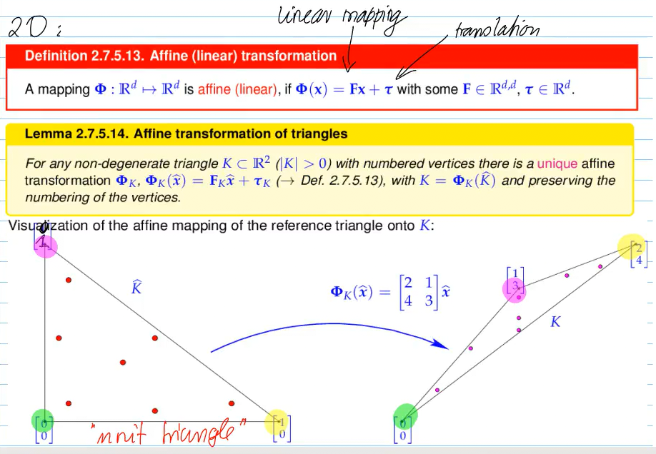
(affine mapping maps lines to lines)

general formula:
Pasted image 20260310135653.png
example on $K \in M$ :
Pasted image 20260310135938.png
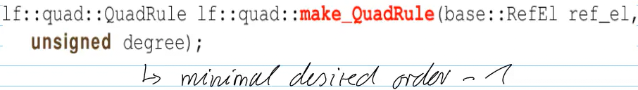
however, if $ϕ_{K}$ affine => $det (D ϕ_{K}) \equiv c o n s t .$ , and we get:
Pasted image 20260310140013.png
in LehrFEM, we can use:
Pasted image 20260310145530.png

Definition 2.7.5.29: Order of a local quadrature rule

A local quadrature rule according to Def. 2.7.5.9 is said to be order $q \in N$ , if

for a simplex $K$ (triangle, tetrahedron) it is exact for all polynomials $f \in P_{q - 1} (R^{d})$ ,
for a tensor product element $K$ (rectangle, brick) it is exact for all tensor product polynomials $f \in Q_{q - 1} (R^{d})$ .

"order $↑ ⟹$ no. of nodes $↑$ "

transformation on affine maps preserves polynomials

-> integral transformation doesn't change order of polynomials

Pasted image 20260310145821.png
quadrature rules in LehrFEM: reference object shape + desired order
Pasted image 20260310145901.png

not copied: code 2.7.5.41: Entity-based composite numerical quadrature

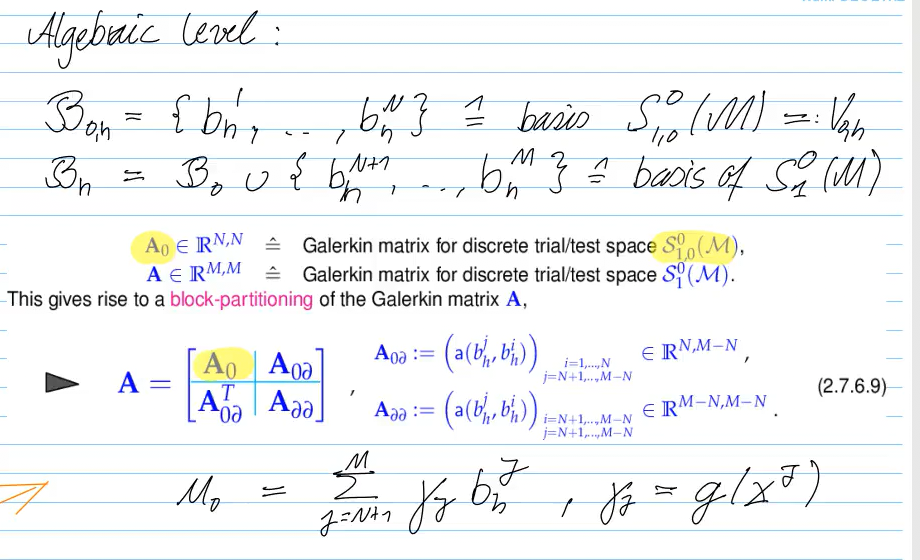
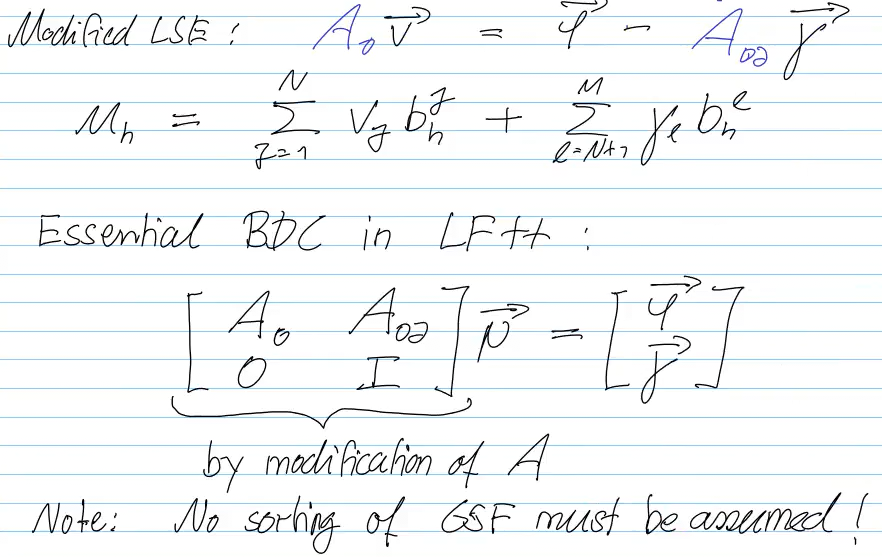
Video 2.7.6 Treatment of Essential Boundary Conditions (21 min)

#todo understand offset function:

Pasted image 20260310150708.png
Pasted image 20260310151152.png
Pasted image 20260310152333.png

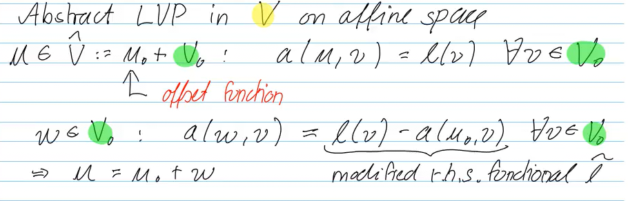
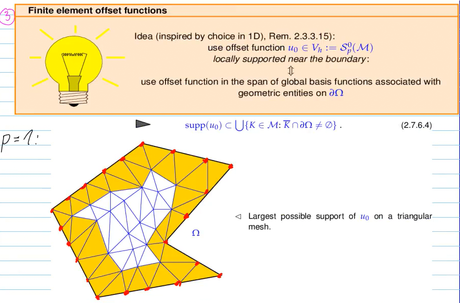
maybe missed something relevant...

Pasted image 20260310152411.png

using LehrFM:
Pasted image 20260310152445.png

not copied code 2.7.6.17: Transformation function, which generates the block matrix from above

Tldr: LehrFEM++ example for dirichlet b.c. problem

Problem: $- Δ u = f$
Weak form: $\int_{Ω} \nabla u \nabla v d x = \int_{Ω} f v d x, \forall v \in H_{0}^{1} (Ω)$

Boundary conditions: Dirichlet (essential)

// 1. Load Mesh and Setup DofHandler for Linear FE (1 DOF per node)
auto factory = std::make_unique<lf::mesh::hybrid2d::MeshFactory>(2);
lf::io::GmshReader readermove(factory), "mesh.msh";
auto mesh_p = reader.mesh();
lf::assemble::UniformFEDofHandler dofh(mesh_p, {{lf::base::RefEl::kPoint(), 1}});

// 2. Prepare Global System Containers (N x N)
lf::assemble::COOMatrix<double> A_triplets(dofh.NumDofs(), dofh.NumDofs());
Eigen::VectorXd rhs = Eigen::VectorXd::Zero(dofh.NumDofs());

// 3. Assemble Stiffness Matrix (using built-in Laplace Provider)
lf::uscalfe::LinearFELaplaceElementMatrix elmat_builder;
lf::assemble::AssembleMatrixLocally(0, dofh, dofh, elmat_builder, A_triplets);

// 4. Handle Dirichlet Boundary Conditions (Offset Function)
auto bd_flags = lf::mesh::utils::flagEntitiesOnBoundary(mesh_p, 2); // Flag nodes
auto selector = [&](unsigned int idx) -> std::pair<bool, double> {
 auto node = dofh.Entity(idx);
 return {bd_flags(*node), 0.0}; // Fix boundary nodes to 0.0
};
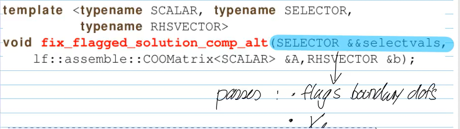
lf::assemble::FixFlaggedSolutionCompAlt(selector, A_triplets, rhs);

// 5. Solve
Eigen::SparseMatrix<double> A = A_triplets.makeSparse();
Eigen::SparseLU<Eigen::SparseMatrix<double>> solver(A);
if(solver.info() != Eigen::Success) abort();
Eigen::VectorXd solution = solver.solve(rhs);

codim: 0->cells, 1->edges, 2->nodes
COOMatrex avoids memory shifts during assembly
AssembleMatrixLocally is templated -> works independent of test/trial space

Video 2.8 Parametric Finite Element Methods I (22 min)

remaining challenge: what to do with general mesh (curved edges, triangles + quadrilaterals)

Affine equivalence
Pasted image 20260314201011.png
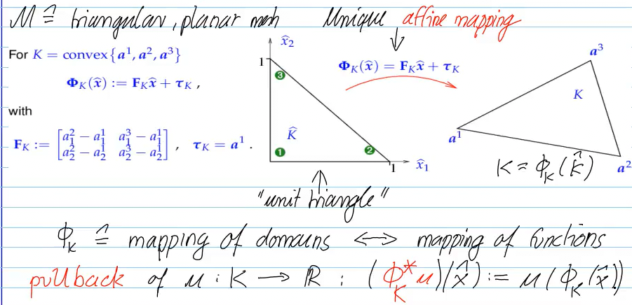
affine pullback preserves polynomials:

Lemma 2.8.1.3: Preservation of polynomials under affine pullback

If $Φ : R^{d} \mapsto R^{d}$ is an affine (linear) transformation ( $\to$ Def. 2.7.5.13), then

Φ^{*} (P_{p} (R^{d})) = P_{p} (R^{d}) and Φ^{*} (Q_{p} (R^{d})) = Q_{p} (R^{d}) .

general quadrilateral lagrangian FE

so far: GSF -> LSF #todo: look this up again
now: start from LSF ${\hat{b}}^{j}$ on reference element $\hat{K}$ -> inverse pullback:

b_{K}^{j} := (ϕ_{K}^{- 1})^{⋆} {\hat{b}}^{j}

-> gluing: GSF

bilinear transformation: componentwise (tensor product) polynomial $\deg = 2$
Pasted image 20260314202207.png

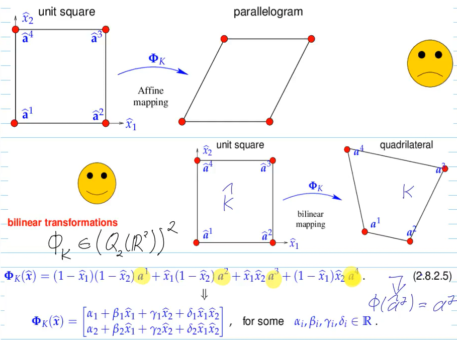
gluing:
-> local shape functions are no longer bilinear, since $ϕ_{K}^{- 1}$ is no longer polynomial (rational function)

Non-polynomial nature of bilinear shape functions

The local shape functions $b_{K}^{i}$ defined by (2.8.2.4), where $Φ_{K}$ is a bilinear transformation and ${\hat{b}}^{i}$ are the bilinear local shape functions on the unit square, are not polynomial in general.

Video2.8 Parametric Finite Element Methods II (27 min)

Pasted image 20260314211639.png
Note that possibility of gluing needs to be checked!

#todo: what are we doing here?

[...]
Pasted image 20260314213531.png
Pasted image 20260314213641.png

Information defining a

H^{1} (Ω)

-conforming parametric finite element

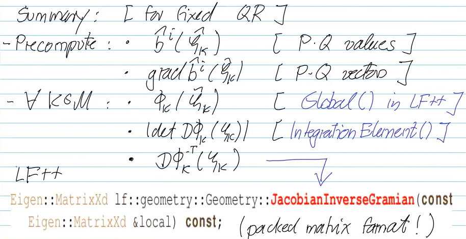
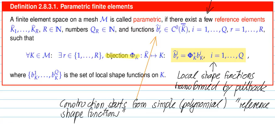
In order to define a $H^{1} (Ω)$ -conforming parametric finite element in a finite element code we have to implement for all reference elements and $i = 1, \dots, Q$

a function realizing $\hat{x} \mapsto {\hat{b}}^{i} (\hat{x}), x \in \hat{K}$ ,
and the evaluation $\hat{x} \mapsto grad {\hat{b}}^{i} (\hat{x}), x \in \hat{K}$ .

// interface in LF++:
size_type ScalarReferenceFiniteElement::NumRefShapeFunctions() const;
size_type ScalarReferenceFiniteElement::NumRefShapeFunctions(dim_t codim) const;
size_type ScalarReferenceFiniteElement::NumRefShapeFunctions(dim_t codim, sub_idx_t subidx) const;

Eigen::Matrix<SCALAR, Eigen::Dynamic, Eigen::Dynamic>
ScalarReferenceFiniteElement::EvalReferenceShapeFunctions(
    const Eigen::MatrixXd& refcoords) const;

Eigen::Matrix<SCALAR, Eigen::Dynamic, Eigen::Dynamic>
ScalarReferenceFiniteElement::GradientsReferenceShapeFunctions(
    const Eigen::MatrixXd& refcoords) const;

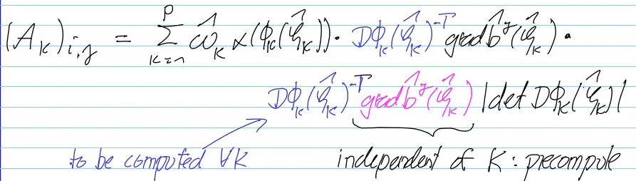
didn't copy code 2.8.3.29: Eval() method for parametric element matrix provider

Boundary Approximation by Parametric FEM:
Pasted image 20260314214831.png
"6-node triangle" in LehrFEM++:
Pasted image 20260314215207.png

Degeneracy of the Transformation

$Φ_{K}$ may be "degenerate" $⟺ D Φ_{K} (\hat{x})$ singular for some $\hat{x} \in \hat{K}$ .

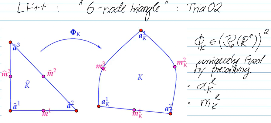
Question: why is this better than simply splitting the curve into multiple triangles? The approximation wouldn't be much worse than by this approach.

3. FEM: Convergence and Accuracy

Video 3.1 Abstract Galerkin Error Estimates (20 min)

convergence (how fast does $u_{h}$ get closer to $μ$ ?) and accuracy (how close is $u_{h}$ to $μ$ ?)

Discretization error $u - u_{h} \in V_{0}$ (a function in BVP context!)

Our goal:

Bound relevant norm of discretization error $u - u_{h}$

A relevant norm:

LVP $⟺ u = \underset{v \in V_{0}}{argmin} J (v), J (v) := \frac{1}{2} a (v, v) - ℓ (v)$ (energy function)

Lemma 3.1.2.3. Energy norm and energy deviation

Let $u \in V_{0}$ solve the linear variational prolem (2.2.0.2),

\begin{matrix} (2.2.0.2) & u \in V_{0} : a (u, v) = ℓ (v) \forall v \in V_{0} \end{matrix}

and let Ass. 3.1.1.2–Ass. 3.1.1.4 be satisfied. Then, with $J (v) := \frac{1}{2} a (v, v) - ℓ (v)$ ,

\begin{matrix} (3.1.2.4) & J (w) - J (u) = ∥ w - u ∥_{a}^{2} \forall w \in V_{0} \end{matrix}

galerkin orthogonality:
Pasted image 20260315120409.png
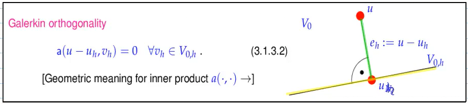
from this follows Pythagoras theorem:
Pasted image 20260315121030.png
Pasted image 20260315121044.png
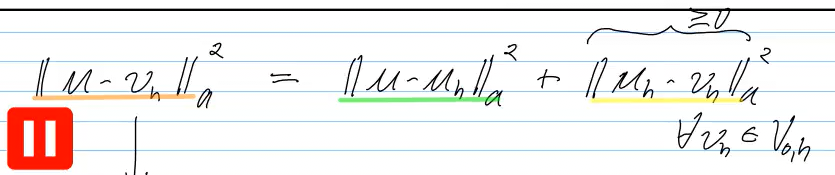
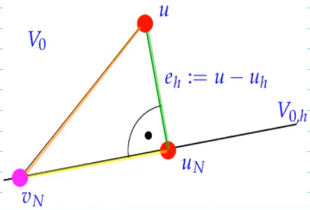
or shorter:

Theorem 3.1.3.7. Cea's lemma

Under Ass. 3.1.1.2–Ass. 3.1.1.4 the energy norm of the Galerkin discretization error for (2.2.0.2) satisfies

∥ u - u_{h} ∥_{a} = inf_{v_{h} \in V_{0, h}} ∥ u - v_{h} ∥_{a} .

-> Galerking solution is optimal (in energy)

minimizes $J (v)$ over $V_{0, h}$

Optimality of Galerkin solutions:

$\begin{matrix} (3.1.3.9) & \underset{((energy) norm of) discretization error}{\underset{⏟}{∥ u - u_{h} ∥_{a}}} = \underset{best approximation error in V_{0, h}}{\underset{⏟}{inf_{v_{h} \in V_{0, h}} ∥ u - v_{h} ∥_{a}}}, \end{matrix}$

-> As regards the energy norm, the Galerkin solution is the best possible solution we can obtain in a given trial space.

Galerking error estimates in energy form approximation error estimates
we can improve the result by enlarging the space (refinement)

Pasted image 20260315121738.png

2d triangular: regular refinement by splitting triangle into 4 congruent triangles
use lf::refinement in LF++

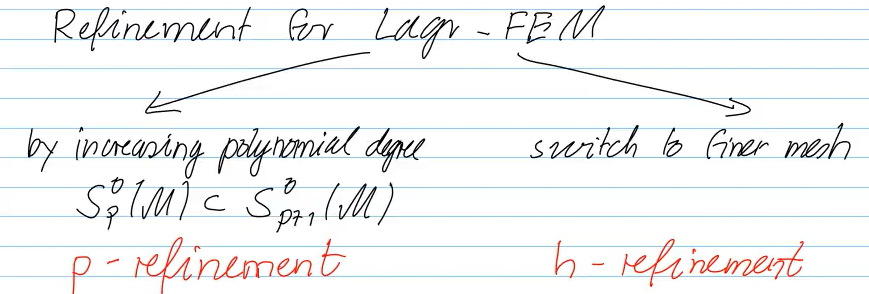
Video 3.2 Empirical (Asymptotic) Convergence of Lagrangian FEM (26 min)

Asymptotic Convergence

Convergence: asymptotic perspective

Crucial: our notion of convergence is asymptotic!
sequence of discrete models $⟹$ sequence of approximate solutions $(u_{h}^{(i)})_{i \in N}$
$↕$ $⟹$ study sequence $(∥ u_{h}^{(i)} - u ∥)_{i \in N}$ as $i \to \infty$
created by variation of a discretization parameter.

Definition 3.2.1.4. Mesh width

Given a mesh $M = {K}$ , its mesh width $h_{M}$ is defined as

h_{M} := max {diam K : K \in M}, diam K := max {| p - q | : p, q \in K} .

limit $h_{m}$ -> 0
for p-refinement, discretication DP $\hat{=}$ degree p

cost might depend on dimension $V_{0, h}$ (or $n n z (A)$ )

algebraic and exponential convergence

Definition 3.2.2.1. Types of convergence

\to

$\begin{aligned} ∥ u - u_{N} ∥ & = O (N^{- α}), α > 0 & ⟺ algebraic convergence with rate α \\ ∥ u - u_{N} ∥ & = O (\exp (- γ N^{δ})), with γ, δ > 0 & ⟺ exponential convergence \end{aligned}$

(asymptotically for $N \to \infty$ )

log-log plot with straigt line: algebraic convergence
lin-log plor with line: exponential convergence

-> (integral) error norms can usually be computed only by numerical quadrature (/sampling) of sufficiently high order

Example:

alg. cvg., but slow convergence for non-smooth solutions (h-refinement)
- $L^{2}$ cvg. seems to be faster than $∥ \cdot ∥_{a}$ -cvg (?)
exp. cvg.(p-refinement)

-> there might be pre-asymptotic behaviour (no convergence until mesh fine / polynomial degree high)

Tldr: h- vs p- refinement

Feature	h-Refinement	p-Refinement
Strategy	Subdivide mesh cells ( $h \to 0$ )	Increase local polynomial degree ( $p \to \infty$ )
Typical Convergence	Algebraic: $O (h^{p})$	Exponential: $O (\exp (- γ p^{δ}))$ for analytic solutions
Limiting Factor	Polynomial degree $p$ and smoothness $k$	Smoothness $k$ of the exact solution
Space Property	Often results in nested spaces (e.g., via regular refinement)	Inherently leads to nested finite element spaces

Video 3.3 A Priori (Asymptotic) Finite Element Error Estimates I (10 min)

Foundation: Cea's lemma

∥ u - u_{h} ∥_{a} = inf_{v_{h} \in V_{0, h}} ∥ u - v_{h} ∥ \leq ∥ u - w_{h} ∥_{a} \forall w_{h} \in V_{0, h}

a suitable "candidate function" $w_{h}$ obtained by interpolation

Note: For 2nd-order elliptic Dirichlet BVP: $∥ v ∥_{a} \sim | v |_{H^{1} (Ω)}$

Global estimates for norms

$\begin{matrix} (3.3.1.14) & | u - I_{1} u |_{H^{1} ([a, b])} \leq h_{M} ∥ u^{″} ∥_{L^{2} ([a, b])} \end{matrix}$

-> algebraic cvg., rate 1

\begin{matrix} (3.3.1.11) & ∥ u - I_{1} u ∥_{L^{2} ([a, b])} \leq h_{M}^{2} ∥ u^{″} ∥_{L^{2} ([a, b])} \end{matrix}

-> algebraic cvg. rate 2

\begin{matrix} (3.3.1.4) & ∥ u - I_{1} u ∥_{L^{\infty} ([a, b])} \leq \frac{1}{4} h_{M}^{2} \underset{smoothness requirement}{\underset{⏟}{∥ u^{″} ∥_{L^{\infty} ([a, b])}}} \end{matrix}

-> algebraic cvg. rate 2

Video 3.3 A Priori (Asymptotic) Finite Element Error Estimates II (18 min)

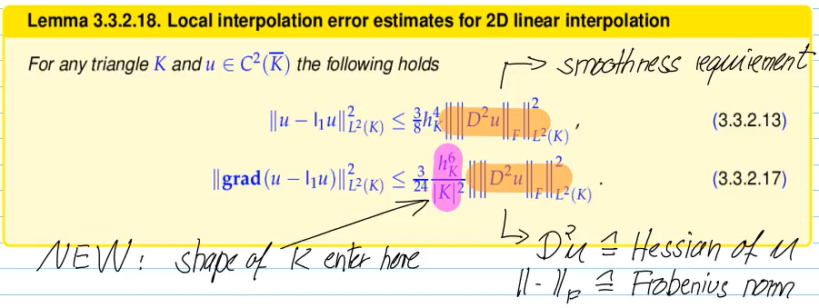
interpolation errors in order to bound the energy norm of the discretization error for lagrangian FEM
still looking for piecewise linear FE, but now in 2D

Definition 3.3.2.1. Linear interpolation in 2D

The linear interpolation operator $I_{1} : C^{0} (\bar{Ω}) \mapsto S_{1}^{0} (M)$ is defined by

I_{1} u \in S_{1}^{0} (M), I_{1} u (p) = u (p) \forall p \in V (M) .

uniquely fixes element of piecweise FE space

Pasted image 20260321201604.png

Definition 3.3.2.20. Shape regularity measure

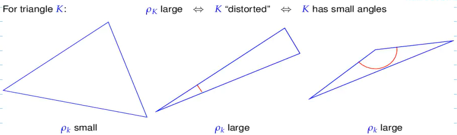
For a simplex $K \in R^{d}$ we define its shape regularity measure as the ratio

ρ_{K} := h_{K}^{d} : | K |

and the shape regularity measure of a simplicial mesh $M = {K}$

ρ_{M} := max_{K \in M} ρ_{K} .

$ρ_{K}$ is similarity-invariant (rotation, scaling, translation)
depends only on it's smallest angle
expresses distortion compared to equilateral triangle $△$ :

Pasted image 20260321202155.png

Theorem 3.3.2.21. Error estimate for piecewise linear interpolation

For any $u \in C^{2} (\bar{Ω})$ and 2D piecewise linear interpolation $I_{1} : C^{0} (\bar{Ω}) \to S_{1}^{0} (M)$ , $M$ a triangular mesh, holds

∥ u - I_{1} u ∥_{L^{2} (Ω)} \leq \sqrt{\frac{3}{8}} h_{M}^{2} ∥ | D^{2} u |_{F} ∥_{L^{2} (Ω)},

-> alg. cvg. rate 2

∥ grad (u - I_{1} u) ∥_{L^{2} (Ω)} \leq \sqrt{\frac{3}{24}} ρ_{M} h_{M} ∥ | D^{2} u |_{F} ∥_{L^{2} (Ω)} .

-> alg. cvg. rate 1
where $h_{M}$ denotes the mesh width ( $\to$ Def. 3.2.1.4) and $ρ_{M}$ the shape regularity measure ( $\to$ Def. 3.3.2.20) of $M$ .

#todo learn multi-index notation

Definition 3.3.3.1. Higher order Sobolev spaces/norms

The $m$ -th order Sobolev norm, $m \in N_{0}$ , for $u : Ω \subset R^{d} \mapsto R$ (sufficiently smooth) is defined by

∥ u ∥_{H^{m} (Ω)}^{2} := \sum_{k = 0}^{m} \sum_{α \in N^{d}, | α | = k} \int_{Ω} | D^{α} u |^{2} d x, where D^{α} u := \frac{\partial^{| α |} u}{\partial x_{1}^{α_{1}} \dots \partial x_{d}^{α_{d}}} .

Sobolev space $H^{m} (Ω) := {v : Ω \mapsto R :== ∥ v ∥_{H^{m} (Ω)} < \infty ==}$ .

$L^{2} (Ω) = H^{0} (Ω) \supset H^{1} (Ω) \supset H^{2} (Ω) \supset H^{3} (Ω) \supset \dots$
$\overset{}{\to}$
increasing regularity of functions

$∥ \cdot ∥_{H^{m}}$ measures "ruggedness" of functions

Definition 3.3.3.3. Higher order Sobolev semi-norms

The $m$ -th order Sobolev semi-norm, $m \in N$ , for sufficiently smooth $u : Ω \mapsto R$ is defined by

| u |_{H^{m} (Ω)}^{2} := \sum_{α \in N^{d}, | α | = m} \int_{Ω} | D^{α} u |^{2} d x .

rewriting error bounds using Sobolev norms, we get:

Corollary 3.3.3.4. Error estimate for piecewise linear interpolation in 2D

Under the assumptions/with notations of Thm. 3.3.2.21 ( $\forall u \in H^{2} (Ω)$ )

\begin{aligned} ∥ u - I_{1} u ∥_{L^{2} (Ω)} & \leq \sqrt{\frac{3}{8}} h_{M}^{2} | u |_{H^{2} (Ω)} \\ | u - I_{1} u |_{H^{1} (Ω)} & \leq \sqrt{\frac{3}{24}} ρ_{M} h_{M} | u |_{H^{2} (Ω)} \end{aligned}

Theorem 3.3.3.8. Sobolev embedding theorem

$m > \frac{d}{2} \Rightarrow H^{m} (Ω) \subset C^{0} (\bar{Ω}) \land \exists C = C (Ω) > 0 : ∥ u ∥_{\infty} \leq C ∥ u ∥_{H^{m} (Ω)} \forall u \in H^{m} (Ω)$

Theorem answers:

"How many derivatives must a function have (in a weak, square-integrable sense) before we can guarantee it is actually a continuous, point-wise defined function?"

e.g. $d = 2$ : m>1 => $H^{2} (Ω)$ functions are guaranteed to be continuous

Video 3.3 A Priori (Asymptotic) Finite Element Error Estimates III (16 min)

Theorem 3.3.5.6. Best approximation error estimates for Lagrangian finite elements

Let $Ω \subset R^{d}, d = 1, 2, 3$ , be a bounded polygonal/polyhedral domain equipped with a mesh $M$ consisting of simplices or parallelepipeds. Then, for each $k \in N$ , there is a constant $C > 0$ depending only on $k$ and the shape regularity measure $ρ_{M}$ such that

inf_{v_{h} \in S_{p}^{0} (M)} ∥ u - v_{h} ∥_{H^{1} (Ω)} \leq C \underset{discretization params.}{\underset{⏟}{{(\frac{h_{M}}{p})}^{min {p + 1, k} - 1}}} \underset{smoothness reqirement}{\underset{⏟}{∥ u ∥_{H^{k} (Ω)}}} \forall u \in H^{k} (Ω) (3.3 .5 .7)

best approximation error $\to$ bounds for FE discretization error for 2nd-order elliptic BVPs (there: $u \hat{=}$ exact solution of BVP) in energy norm
"generic constant":
- actual value unknown
- dependence known

If we assume uniform shape-regularity and local quasi-uniformity of the mesh, then, from theorem 3.3.5.6 we get:

\begin{matrix} (3.3.5.19) & inf_{v_{h} \in S_{p}^{0} (M)} | u - v_{h} |_{H^{1} (Ω)} \leq C N^{- \frac{min p, k - 1}{d}} | u |_{H^{k} (Ω)} \end{matrix}

=> Algebraic convergence of discretization error with respect to N (DOFs), rate

\frac{1}{d} min (p, k - 1)

rate limited by
- polynomial degree $p$
- smoothness
rate deteriorates for larger $d$

By what extra cost can we buy a certain improvement of the FEM solution? (3.3.5.23)

Assuming the a priori error estimate is sharp (the actual error follows the theoretical trend), the relationship between error reduction and computational cost is:

The Goal (Gain): Reduce the discretization error (energy norm) by a factor of $ρ > 1$ .
The Price (Cost): Increase the number of unknowns ( $N$ ) by a factor of: $$\text{Cost Factor} \approx \rho^{\frac{d}{\min{p, k-1}}}$$

takeaways

The Curse of Dimension ( $d$ ): As the spatial dimension $d$ increases, the cost of reducing error grows exponentially. Accuracy is much "cheaper" in 1D than in 3D.
Optimal Efficiency ( $p = k - 1$ ): For best gain/cost, polynomial degree $p$ should match solution's smoothness $k$ ( $H^{k}$ )
Smoothness Matters: For very smooth solutions ( $k$ is large), high-order elements ( $p > 1$ ) reduce the required increase in $N$ significantly compared to linear elements ( $p = 1$ ).
The "Slow" Limit: If the solution is not smooth (small $k$ ), increasing the polynomial degree $p$ does not help efficiency, because the cost factor will be stuck at $ρ^{d / (k - 1)}$ regardless of how high you choose $p$ .

type of refinement	alg. cvg. rate
h-refinement ( $p$ fixed & small: $p \leq k - 1$ )	$- p / d$
h-refinement (low regularity of u: $k \leq p + 1$ )	$- (k - 1) / d$
p-refinement ( $h_{m}$ fixed, limited regularity $u$ )	$- (k - 1) / d$
p-refinement (perfectly smooth (analytic) solution) (because $C$ depends on $k$ in unspecified way)	theorem doesn't work

Here is a compressed summary of Unit 3.3 for your markdown callout, based on the course videos and documents:

Tldr 3.3: A Priori Finite Element Error Estimates

Cea's Lemma: energy norm of discretization $\hat{=}$ best approximation error of FE space
accuracy is governed by the mesh width ( $h_{M}$ ), the polynomial degree ( $p$ ), and the Sobolev smoothness ( $u \in H^{k}$ ) of the exact solution.

General $H^{1}$ -Error Estimate:

inf_{v_{h} \in S_{p}^{0} (M)} | u - v_{h} |_{H^{1} (Ω)} \leq C {(\frac{h_{M}}{p})}^{min {p, k - 1}} | u |_{H^{k} (Ω)} $ $ w h e r e t h e g e n e r i c c o n s t a n t $ C $ d e p e n d s o n t h e * * s h a p e r e g u l a r i t y * * ($ ρ_{M} $) o f t h e m e s h b u t i s i n d e p e n d e n t o f $ h_{M} $ . * * A l g e b r a i c C o n v e r g e n c e T r e n d s ($ h $ - r e f i n e m e n t) : * * O n q u a s i - u n i f o r m m e s h e s, t h e e r r o r d e c a y s r e l a t i v e t o t h e n u m b e r o f u n k n o w n s ($ N $) a s : $ $ Error Norm (N) \approx C N^{- α}, with rate α = \frac{min {p, k - 1}}{d}

Curse of Dimension: Convergence speed deteriorates as the spatial dimension $d$ increases.
Rate Limits: The rate is limited by either the polynomial degree $p$ (for smooth solutions) or the solution's lack of regularity $k$ (for rough solutions).

Asymptotic Efficiency (Cost-Benefit): Reducing the error by a factor $ρ > 1$ requires increasing the problem size $N$ by a factor of $ρ^{d / min p, k - 1}$ . Efficiency is theoretically optimal when $p = k - 1$ .

#todo Learn more about Sobolev regularity (solution $u \subset H^{k} (Ω)$ , which $k$ ?)

Video 3.4 Elliptic Regularity Theory (11 min)

WHat is the Sobolev regularity of solutions of elliptic BVP?

Theorem 3.4.0.2. Smooth elliptic lifting theorem

If $\partial Ω$ is $C^{\infty}$ -smooth, ie. possesses a local parameterization by $C^{\infty}$ -functions, and $σ \in C^{\infty} (\overset{―}{Ω})$ , then, for any $k \in N$ ,

\begin{aligned} Dirichlet problem & u \in H_{0}^{1} (Ω) and - div (σ grad u) \in H^{k} (Ω) \\ Neumann prob. & u \in H^{1} (Ω), - div (σ grad u) \in H^{k} (Ω) and grad u \cdot n = 0 on $ \partial Ω \end{aligned}

$\Rightarrow u \in H^{k + 2} (Ω)$ .

In addition, for such $u$ there is $C = C (k, Ω, σ)$ such that

∥ u ∥_{H^{k + 2} (Ω)} \leq C ∥ div (σ grad u) ∥_{H^{k} (Ω)}

probably irrelevant:

Theorem 3.4.0.6. Corner singular function decomposition

Let $Ω \subset R^{2}$ be a polygon with $J$ corners $c^{i}$ . Denote the polar coordinates in the corner $c^{i}$ by $(r_{i}, φ_{i})$ and the inner angle at the corner $c^{i}$ by $ω_{i}$ . Additionally, let $f \in H^{l} (Ω)$ with $l \in N_{0}$ and $l \neq λ_{i k} - 1$ , where the $λ_{i k}$ are given by the singular exponents

\begin{matrix} (3.4.0.7) & λ_{i k} = \frac{k π}{ω_{i}} for k \in N . \end{matrix}

Then $u \in H_{0}^{1} (Ω)$ with = $- Δ u = f$ = in $Ω$ (Dirichlet prob.) can be decomposed

\begin{matrix} (3.4.0.8) & u = u^{0} + \sum_{i = 1}^{J} ψ (r_{i}) \sum_{λ_{i k} < l + 1} κ_{i k} s_{i k} (r_{i}, φ_{i}), κ_{i k} \in R, \end{matrix}

with regular part $u^{0} \in H^{l + 2} (Ω)$ , cut-off functions $ψ \in C^{\infty} (R^{+})$ ( $ψ \equiv 1$ in a neighborhood of $0$ ), and corner singular functions

\begin{matrix} (3.4.0.9) & \begin{aligned} λ_{i k} \notin N : & s_{i k} (r, φ) = r^{λ_{i k}} \sin (λ_{i k} φ), \\ λ_{i k} \in N : & s_{i k} (r, φ) = r^{λ_{i k}} (\ln r) \sin (λ_{i k} φ) . \end{aligned} \end{matrix}

=> reentrant corners lead to very poor regularity

Intermediate

$Ω \subset R^{2}$ has re-entrant corners $⟹$ if $u$ solves $Δ u = f$ in $Ω$ , $u = 0$ on $\partial Ω$ , then $u \notin H^{2} (Ω)$ in general.

however, for convex problems, the dirichlet solution is in $H^{2}$ (BVP is 2-regular)

Theorem 3.4.0.10. Elliptic lifting theorem on convex domains

If $Ω \subset R^{d}$ convex, $u \in H_{0}^{1} (Ω), Δ u \in L^{2} (Ω) \Rightarrow u \in H^{2} (Ω)$ .

Video 3.5 Variational Crimes (15 min)

"theory is incredibly difficult"

Variational crime: instead of solving exact discrete variational problem, we solve a perturbed one:

a_{h} ({\tilde{u}}_{h}, v_{h}) = l_{h} (v_{h})

-> inevitable, since some functions are only given in procedural form

Guideline for acceptable variational crimes

Variational crimes must not affect (type and rate) of asymptotic convergence

Impact of Numerical Quadrature

Note: To show that QR is of order 2 -> show that it integrates polybomials of order 1 exactly (n-1) -> integrates $λ_{1}, λ_{2}, λ_{3}$ exactly

Intermediate

Finite element theory tells us that the above guideline can be met, if the local numerical quadrature rule has sufficiently high order. The quantitative results can be condensed into the following rules of thumb:

Target Accuracy	Required Quadrature Order
$\| u - u_{h} \|_{1} = O (h_{M}^{p})$	Order $2 p - 1$ sufficient for $f_{h}$
$\| u - u_{h} \|_{1} = O (h_{M}^{p})$	Order $2 p - 1$ sufficient for $a_{h}$

Example of crime: Using midpoint rule (order 2) for quadratic elements ( $p = 2$ ) will cause convergence rate in terms of $N$ to drop.

Impact of boundary approximation

Rule of thumb deduced from sophisticated finite element theory:

If $V_{0, h} = S_{p}^{0} (M)$ , use boundary fitting with polynomials of degree $p$ .

for quadratic FEM, use quadratic boundary approximation (see chapter 2)

Example of crime: When $Ω$ has curved boundary, approximation with polygon (linear) is a crime (perturbed domain $Ω_{h}$ )

When using LehrFEM to refine meshes, the boundary stays the same -> round boundary does not get "rounded" when refining

Video 3.8 Validation and Debugging of Finite Element Codes (13 min)

matching theoretical rates are a strong circumstatial evidence of correctness

-> if code converges mroe slowly than theory predicts, there is almost certainly a bug

3 main methods:

observing convergence between mesh levels

test code by comparing solutions on a sequence of nested meshes created by regular refinement

refine mesh -> $| u_{k} - u_{k - 1} |$ should shrink
norm of the difference, $| | u_{k} - u_{k - 1} | |$ should display the same algebraic convergence rate ( $α$ ) as the actual discretization error
shortcut: compare the difference of their norms ( $| | | u_{k} | | - | | u_{k - 1} | | |$ ), should also converge at rate $α$

method of manufactured solutions

6. Second-Order Linear Evolution Problems

Video 9.2.1 Heat Equation (10 min)

linear evolution: time-dependent / transient
posed on space-time cylinder

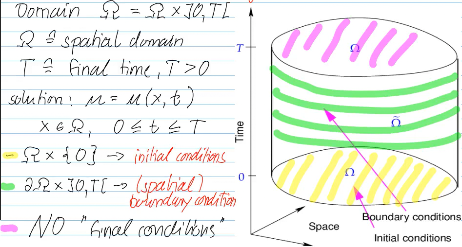
6.2 Parabolic Initial-Boundary Value Problems

balance law:
Pasted image 20260328150854.png
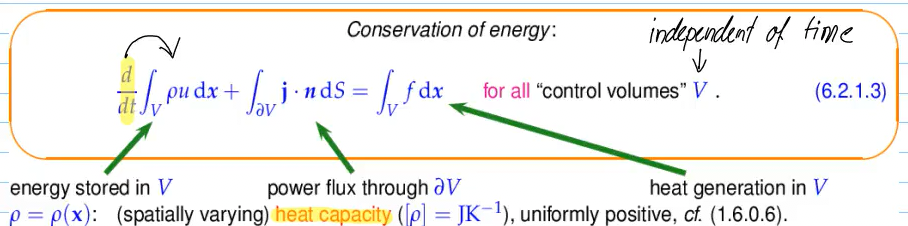
using localization and fourier law, we get:

\frac{\partial}{\partial t} (ρ u) - div (κ (x) grad u) = f in \tilde{Ω} := Ω \times] 0, T [

spatial b.c.:

For second order parabolic evolutions we can/must use the same spatial boundary conditions as for stationary second order elliptic boundary value problems

(although the boundary conditions are now dependent from x and t)

initial conditions (temporal b.c.):

u (x, 0) = u_{0} (x) BVP

combined:

\begin{aligned} (7.1.1.5) & \frac{\partial}{\partial t} (ρ (x) u) - div (κ (x) grad u) & = f in \tilde{Ω} := Ω \times] 0, T [, \\ (7.1.1.7) & u (x, t) & = g (x, t) for (x, t) \in \partial Ω \times] 0, T [, \\ (7.1.1.8) & u (x, 0) & = u_{0} (x) for all x \in Ω . \end{aligned}

Video 9.2.2 Heat Equation: Spatial Variational Formulation (8 min)

Spatial variational form of (7.1.1.5)–(7.1.1.7): seek $t \in] 0, T [\mapsto u (t) \in H_{0}^{1} (Ω)$

\begin{aligned} (6.2.2.4) & \underset{=: m (\dot{u}, v)}{\underset{⏟}{\int_{Ω} ρ (x) \dot{u} (t) v d x}} + \underset{=: a (u (t), v)}{\underset{⏟}{\int_{Ω} κ (x) \nabla u (t) \cdot \nabla v d x}} & = \underset{=: l (v)}{\underset{⏟}{\int_{Ω} f (x, t) v (x) d x}} \forall v \in H_{0}^{1} (Ω), \\ (6.2.2.5) & initial condition ⟶ u (0) & = u_{0} \in H_{0}^{1} (Ω) \end{aligned}

abstract linear evolution problem:

\begin{array}{r} (6.2.2.8) & t \in] 0, T [\mapsto u (t) \in V_{0} : {\begin{cases} m (\dot{u} (t), v) + a (u (t), v) = ℓ (t) (v) \forall v \in V_{0}, \\ u (0) = u_{0} \in V_{0} . \end{cases} \end{array}

a, m are independent of time and s.p.d
solution will depend linearly on f, $u_{0}$

Video 9.2.3 Stability of Parabolic Evaolution Problems (10 min)

It is always simpler to look at the square of the norms

reminder: Poincare-Friedrichs inequality:

γ \underset{= L^{2} - norm}{\underset{⏟}{∥ v ∥_{m}^{2}}} \leq \underset{\sim H^{1} - seminorm}{\underset{⏟}{∥ v ∥_{a}^{2}}} \forall v \in V_{0}

Lemma 6.2.3.3. Decay of solutions of parabolic evolutions

For $f \equiv 0$ the solution $u (t)$ of (7.1.2.4) satisfies

∥ u (t) ∥_{m} \leq e^{- γ t} ∥ u_{0} ∥_{m}, ∥ u (t) ∥_{a} \leq e^{- γ t} ∥ u_{0} ∥_{a} \forall t \in] 0, T [

where $γ > 0$ is the constant from (7.1.3.1), and $∥ \cdot ∥_{a}$ , $∥ \cdot ∥_{m}$ stand for the energy norms induced by $a (\cdot, \cdot)$ and $m (\cdot, \cdot)$ , respectively.

Dissipation of energy in parabolic evolutions

Exponential decay of energy during parabolic evolution without excitation ("Parabolic evolutions dissipate energy")

Video 9.2.4 Spatial Semi-Discretization: Method of Lines (6 min)

-> spatial Galerkin discretization of 6.2.2.8 yields:

\sum_{i = 1}^{N} {\dot{μ}}_{i} (t) m (b_{h}^{i}, b_{h}^{j}) + \sum μ_{i} (t) a (b_{h}^{i}, b_{h}^{j}) = ℓ (t) (b_{h}^{j}) \forall v_{h} \in V_{0, h}, j = 1, \dots, N

Method-of-lines ordinary differential equation

Combining (7.1.4.1) and (7.1.4.2) we obtain

\begin{matrix} (6.2.4.4) & (7.1 .4 .1) \Rightarrow {\begin{cases} M {\frac{d}{d t} \vec{μ} (t)} + A \vec{μ} (t) = \vec{φ} (t) \\ \vec{μ} (0) = {\vec{μ}}_{0} \end{cases} for 0 < t < T, \end{matrix}

with

s.p.d. stiffness matrix $A \in R^{N, N}$ , $(A)_{i j} := a (b_{h}^{j}, b_{h}^{i})$ (independent of time),
s.p.d. mass matrix $M \in R^{N, N}$ , $(M)_{i j} := m (b_{h}^{j}, b_{h}^{i})$ (independent of time),
source (load) vector $\vec{φ} (t) \in R^{N}$ , $(\vec{φ} (t))_{i} := ℓ (t) (b_{h}^{i})$ (time-dependent),
${\vec{μ}}_{0} ≜$ coefficient vector of a projection of $u_{0}$ onto $V_{0, h}$ .

Note

(7.1.4.4) is an ordinary differential equation (ODE) for $t \mapsto \vec{μ} (t) \in R^{N}$

but only semi-discretization, since $\vec{μ} (t)$ is still function of continuous time

=> MOL-ODE is semi-discrete

Video 9.2.7 Timestepping for Method-of-Lines ODE (30 min)

\begin{aligned} (7.1.7.2) & Expl. Eul. (7.1.7.2): & {\vec{μ}}^{(j)} = {\vec{μ}}^{(j - 1)} + τ_{j} M^{- 1} (\vec{φ} (t_{j - 1}) - A {\vec{μ}}^{(j - 1)}) \\ (7.1.7.3) & Impl. Eul. (7.1.7.3): & {\vec{μ}}^{(j)} = (τ_{j} A + M)^{- 1} (M {\vec{μ}}^{(j - 1)} + τ_{j} \vec{φ} (t_{j})) \end{aligned}

since s.p.d., can be invertedy -> use Cholesky-decomposition ( #todo what is that?)

MOL-ODE is stiff!

Explicit Euler timestepping is not stable (exponential blow-up) in case of large timestep combined with fine mesh.

Lemma 6.2.7.32. Behavior of generalized eigenvalues

Let $M$ be a simplicial mesh and $A$ , $M$ denote the Galerkin matrices for the bilinear forms $a (u, v) = \int_{Ω} grad u \cdot grad v d x$ and $m (u, v) = \int_{Ω} u (x) v (x) d x$ , respectively, and $V_{0, h} := S_{p, 0}^{0} (M)$ . Then the smallest and largest generalized eigenvalues of $A \vec{μ} = λ M \vec{μ}$ , denoted by $λ_{min}$ and $λ_{max}$ , satisfy

\frac{1}{diam (Ω)^{2}} \leq λ_{min} \leq C, λ_{max} \geq C h_{M}^{- 2},

where the "generic constants" ( $\to$ Rem. 3.3.5.10) depend only on the polynomial degree $p$ , the domain $Ω$ , and the shape regularity measure $ρ_{M}$ .

-> timestep constraint: $τ \leq C h_{m}^{2}$ (similar to ode45)

diagonalization of RK-SSM ( $\vec{φ} \equiv 0$ )
Pasted image 20260328180532.png

Unconditional stability of single step methods

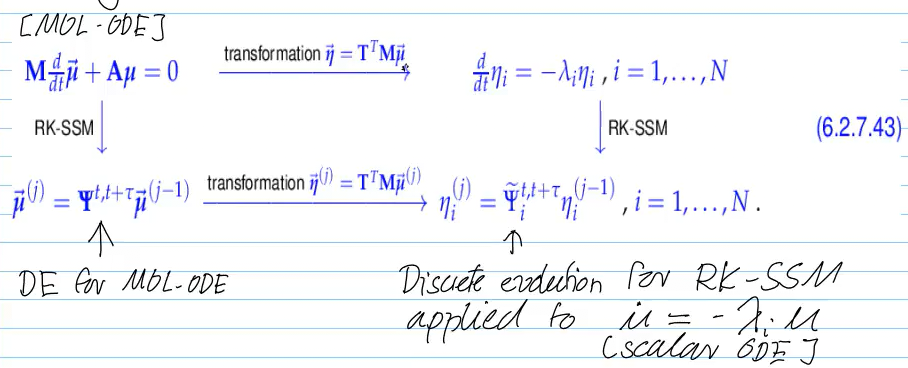
Necessary condition for $universal unconditional stability$ of a single step method for semi-discrete parabolic evolution problem (7.1.4.4) ("method of lines"):

The discrete evolution $Ψ_{λ}^{τ} : R \mapsto R$ of the single step method applied to the scalar ODE $\dot{u} = - λ u$ satisfies

\begin{matrix} (6.2.7.45) & λ > 0 ⟹ lim_{j \to \infty} (Ψ_{λ}^{τ})^{j} u_{0} = 0 \forall u_{0} \in R, \forall τ > 0. \end{matrix}

RK-SSM for $\dot{u} = - λ u \Rightarrow u^{(j)} = \underset{stability functions}{\underset{⏟}{S (- λ τ)}} u^{(j - 1)}$

\begin{array}{cc} c & A \\ b^{⊤} \end{array}

\Psi^{t, t+\tau}_\lambda u = \textcolor{yellow}{S(-\lambda \tau)} u, \tag{6.2.7.47a}$$with rational stability function $$\textcolor{yellow}{S(z)} = 1 + z\textcolor{orange}{\mathbf{b}}^\top (\mathbf{I} - z\textcolor{green}{\mathfrak{A}})^{-1} \mathbf{1} = \frac{\det(\mathbf{I} - \textcolor{yellow}{z}\textcolor{green}{\mathfrak{A}} + z\mathbf{1}\textcolor{orange}{\mathbf{b}}^\top)}{\det(\mathbf{I} - z\textcolor{green}{\mathfrak{A}})}, \quad \mathbf{1} = [1, \dots, 1]^\top \in \mathbb{R}^s. \tag{6.2.7.47b}

$\to$ a rational function in $z$

RK-SSM is unconditionally stable for MOL-ODE if $| S (z) | \leq 1 \forall z < 0$

evne desirable $| S (z) | ≪ 1$ for $z < 0$

Definition 6.2.7.48. L(

π

)-stability

A Runge-Kutta single-step method satisfying (7.1.7.45) is called $L (π) -stable$ , if its stability function $S (z)$ according to (7.1.7.47b) satisfies

$| S (z) | < 1$ for all $z < 0$ , and
" $S (- \infty)$ " $:= lim_{z \in R \to - \infty} S (z) = 0$ .

Pasted image 20260328181937.png
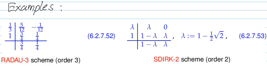
necessarily implicit

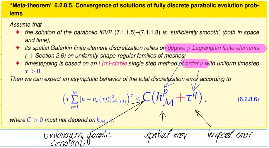
Video 9.2.8 Fully Discrete Method of Lines: Convergence (18 min)

The Parabolic Discretization Path

Heat Equation (Strong Form): transient heat equation on a space-time cylinder $Ω \times] 0, T [$ , subject to initial and boundary conditions: $\frac{\partial u}{\partial t} - Δ u = f (x, t) in Ω, u (x, t) = 0 on \partial Ω$
Spatial Variational Formulation: By treating time $t$ as a passive parameter and applying integration by parts in the spatial domain, the PDE is converted to a weak form:

\int_{Ω} \frac{\partial u}{\partial t} v d x + \int_{Ω} grad u \cdot grad v d x = \int_{Ω} f (t) v d x \forall v \in H_{0}^{1} (Ω)

Abstract Formulation: The weak form is generalized into an abstract parabolic evolution problem using the mass bilinear form $m (\cdot, \cdot)$ and the stiffness bilinear form $a (\cdot, \cdot)$ :

m (\dot{u}, v) + a (u, v) = ℓ (t) (v) \forall v \in V_{0}

Method of Lines ODE: Applying Galerkin discretization in space (e.g., using finite elements) transforms the abstract evolution into a system of ordinary differential equations for the coefficient vector $\vec{μ} (t)$ :

M \dot{\vec{μ}} (t) + A \vec{μ} (t) = \vec{φ} (t)

where $M$ is the mass matrix and $A$ is the stiffness matrix.
5. Runge-Kutta Method (Full Discretization): Finally, the semi-discrete ODE is integrated in time using a single-step method (SSM). For parabolic problems, L-stable Runge-Kutta methods (such as Radau methods) are preferred to ensure stability:

{\vec{μ}}^{(j)} = Ψ_{τ, t_{j - 1}} {\vec{μ}}^{(j - 1)}

resulting in a fully discrete scheme where the total error is the combined effect of spatial and temporal discretization.

Pasted image 20260328195207.png

Refinement for fully discrete parabolic evolution problems

Guideline: spatial and temporal resolution have to be adjusted in tandem

for a conditionally stable explicit method, we often have timestep constraint $τ \leq C h^{2}$

-> if we reduce mesh for accuracy, we have to reduce the timestep more severly than accuarcy requires -> inefficiency "overkill constraint"

-> use unconditionally stable implicit methods instead

We're converting image into markdown + latex formulas. For normal text, normal markdown. For boxes, use callouts. The format of callouts is the following:

> [!name] <title>
> content

Note that there is no empty line between the callout header and the content!

orange boxes: convert to !intermediate
lemmas, theorems (yellow): convert to !lemma, !theorem
definitions (red): convert to !definition

Highlighted text can be highlighted in markdown, too: =highlight. This is not standard commonmark, but if you see highlighted text in the image, highlight it when converting, too. Same for bold: if a text is emphasised, make it bold.
-> Note that hihglighting can only be used for markdown, not for latex
-> If something cannot be converted to pure markdown, warn me instead of attempting to use non-standard syntax.
-> For this task, you may omit any custom formats specified earlier.
-> Your answer should consist solely of the markdown (and the warning if something cannot be converted). No follow-up suggestions, questions, clarifications.
-> for colors in latex, use \textcolor{color}{content} instead of \color{color}{content}